Predication of 3-D Viscous Flowfield of a Centrifugal Impeller

doi:10.4236/epe.2011.31005

Paper Menu >>

Journal Menu >>

Energy and Power En gi neering, 2011, 3, 29-33

doi:10.4236/epe.2011.31005 Published Online February 2011 (http://www.SciRP.org/journal/epe)

Predication of 3-D Viscous Flowfield of a Centrifugal

Impeller

Limin Gao, Xudong Feng, Jian Xie

School of Power and Energy, Northwestern Polytechnical University, Xi’an, China

E-mail: [email protected]

Received September 10, 2010; revised November 5, 2010; accepted November 15, 2010

Abstract

A three-dimensional viscous code has been developed to solve Reynolds-averaged Navier-Stokes equations.

The governing equations in finite volume form are solved by two-step Runge-Kutta scheme with implicit

residual smoothing. The eddy viscous is obtained using the Baldwin-Lomax model. A prediction of the 3-D

turbulent flow and the performance in the “all-over controlled vortex distribution” centrifugal impeller with a

vaneless diffuser has been made for the compressor at design and off-design condition. The predicted effi-

ciency is a little higher than the experiment data. These results suggest that the present calculation code is

able to determine the flow development in the impeller and also the turbulence model in the centrifugal im-

peller should be improved.

Keywords: Centrifugal Impeller, Aerodynamic Performance, 3-D Viscous Flow Calculation, Design &

off-Design Conditions

1. Introduction

Centrifugal compressors are used widely in industry due

to their advantages of simple structure and high-pressure

ratio. However, their efficiency and stability are ad-

versely influenced by the present of impeller exit flow

non-uniformity. In recent years, as a result of improve-

ments in experimental techniques and numerical methods,

it has been possible to avoid the non-uniformity of exit

flow field in order to obtain improved efficiency and

stability of an impeller. The work of Eckardt’s [1] and

Krain’s [2] are most representative in all related experi-

mental research. Their studies indicated that both com-

plicated secondary flows and separated boundary layer

would cause the radial and circumferential non-uniform

flows at the outlet, and consequently the performance of

the centrifugal compressor decreases. Meanwhile, some

numerical codes have also been developed to study the

flowfield in centrifugal compressor by other researchers.

Most of them [2-4] have provided the detailed flowfield

to understand the complicated flow. However, CFD is

still a little immature and does not reach the engineering

implementation level. Further research is necessary to

develop a more accurate and faster, numerical predicting

code, which will provide the sophisticated tool to predict

the aerodynamic performance of a high-speed centrifugal

compressor for designing an impeller with higher pres-

sure-ratio and efficiency.

In the present work, a 3-D turbulent code has been

developed, and the prediction of 3-D viscous flowfield of

an AOCV centrifugal impeller has been carried out.

Therefore, it is hoped that the present study will provide

a useful predication tool to aid in the future experimental

work and the industrial design.

2. AOCV Centrifugal Impeller

The air compressor, which is applied in a large-scale

air-separation plant, is produced from SER Turboma-

chinery Research Center of the Xi’an JiaoTong Univer-

sity. Its impeller is a three-dimensional centrifugal im-

peller which is design using the All-Over Controlled

Vortex Distribution designing theory.

The impeller is shrouded and has 19 full blades with

an exit backswept of 50 degs. The inlet diameter is 0.222

m and the inlet blade height is 0.0606m. The exit diame-

ter is 0.340 m and the exit blade height is 0.0272 m. The

design speed of 16360 rpm gives a rotor exit tip speed of

290 m/s. The design mass flow rate is 2.8 m3/s at the

standard inlet conditions of 101, 325 N/m2 and 288.15 K.

The rotor tip Reynolds number (U2D2/ν) is 1.42 × 106.

The impeller is showed in Figure 1.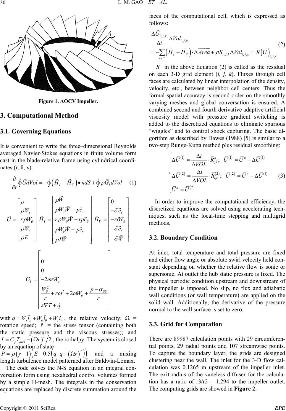

L. M. GAO ET AL.

Figure 1. AOCV Impeller.

3. Computational Method

3.1. Governing Equations

It is convenient to write the three–dimensional Reynolds

averaged Navier-Stokes equations in finite volume form

cast in the blade-relative frame using cylindrical coordi-

nates (r, θ, x):



IV I

UdVolHHndSG dVol



 

 







 

(1)

WW pe

UrWH rWWrpeHre

WW pe

















 



 



 







 







 



 



 













 













GrW





















 



















with ˆˆ

qWi WiWi





, the relative velocity; Ω =

rotation speed;







= the stress tensor (containing both

the static pressure and the viscous stresses); and

porel

ICT r, the rothalpy. The system is closed

by an equatio

and a mixing

length turbulence model patterned after Baldwin-Lomax.

n state



.PE











5qq



The code solves the N-S equation in an integral con-

versation form using hexahedral control volumes formed

by a simple H-mesh. The integrals in the conservation

equations are replaced by discrete summation around the

faces of the computational cell, which is expressed as

follows:

 

,, ,,,,

ijk ijk

IVijk ijkijk

cell

UVol

HHArea SVolRU







 







(2)



in the above Equation (2) is called as the residual

on each 3-D grid element (i, j, k). Fluxes through cell

faces are calculated by linear interpolation of the density,

velocity, etc., between neighbor cell centers. Thus the

formal spatial accuracy is second order on the smoothly

varying meshes and global conversation is ensured. A

combined second and fourth derivative adaptive artificial

viscosity model with pressure gradient switching is

added to the discretized equations to eliminate spurious

“wiggles” and to control shock capturing. The basic al-

gorithm as described by Dawes (1988) [5] is similar to a

two-step Runge-Kutta method plus residual smoothing:

  

  



222

;

ijk

URUU

VOL

URUU

VOL



 







 









(3)

In order to improve the computational efficiency, the

discretized equations are solved using accelerating tech-

niques, such as the local-time stepping and multigrid

methods.

3.2. Boundary Condition

At inlet, total temperature and total pressure are fixed

and either flow angle or absolute swirl velocity held con-

stant depending on whether the relative flow is sonic or

supersonic. At outlet the hub static pressure is fixed. The

physical periodic condition upstream and downstream of

the impeller is imposed. No slip, no flux and adiabatic

wall conditions (or wall temperature) are applied on the

solid wall. Additionally, the derivative of the pressure

normal to the wall surface is set to zero.

3.3. Grid for Computation

There are 89987 calculation points with 29 circumferen-

tial points, 29 radial points and 107 streamwise points.

To capture the boundary layer, the grids are designed

clustering near the wall. The inlet for the 3-D flow cal-

culation was 0.1265 m upstream of the impeller inlet.

The exit radius of the vaneless diffuser for the calcula-

tion has a ratio of r3/r2 = 1.294 to the impeller outlet.

The computing grids are showed in Figure 2.

L. M. GAO ET AL.

ing requirements are satisfied: 1) the mass flow error

throughout the domain was deemed acceptable and flow

mass in inlet and outlet are in accordance, 2) both

RMSM (maximum computing error, which is expressed

as Equation (4)) and RMS (summation of computing

error, which is expressed as Equation (5)) through all

computing points decrease three or four orders; 3) the

flow variables (velocity or pressure) at the arbitrary

computational point is monitored to insure that the ve-

locity field was not changing.

4. Results of 3-D Prediction

The predicated meridional velocity vectors on three sur-

faces with three tangential positions are presented in

Figure 2. There is no backflow at the diffuser exit and

no separation in the shroud boundary layer all through

the compressor. Flow near the pressure side of the im-

peller passage is shown in Figure 3(a). A secondary

flow from the hub to shroud becomes evident in the sec-

ond half of the passage due to curvature of the passage

from the axial to radial direction. At mid-passage, Fig-

ure 3(b) shows the shroud boundary layer is thickening

in impeller and velocity vectors are nearly parallel to the

shroud and the hub. Near the suction side of the impeller,

centrifugal and curvature effects combine to give strong

secondary flows towards the shroud. This is especially

true in the second half of the passage, where flow angles

as high as 30 degs to the meridional direction is seen in

Figure 3(c). Clearly the meridional velocity near the

suction surface is larger than near the pressure surface.

(a)

Distribution of the static pressure on the mid-pitch

meridional surface through the impeller is presented on

the Figure 4. The value on the pressure contours is the

ratio of the local static pressure to the inlet total pressure.

From the Figure 4, it can be seen that the static pressure

is gradually increased and that the distribution of the

static pressure is uniform comparatively on the same

chord section.

(b)

Figure 2. Grid for 3-D flow computation, (a) Meridional

view; (b) Blade-to-blade plane near impeller leading edge. The measured and calculated total/total polytropic

impeller efficiency is presented on Figure 5. In the cal-

culation, the centrifugal impeller works on the design

and the off-design conditions at 100 percent design speed

respectively, totally eight work-conditions. According to

3.4. Convergence

Computing convergence is determined when the follow-

ijk

VV e

RMSM Maxtttt t

















 





 





 

 





(4)

,, 1,,

IM JM KMzr

ijk ijk

VV e

tttt t

RMS IM JM KM



















 





 





 

 









(5)

L. M. GAO ET AL.

(a)

(b)

Figure 4. static pressure contour on the mid-pitch surface.

Figure 5. performance map of the AOCV centrifugal im-

peller.

cient

the experiment, the y-axis is the impeller polytropic effi-













 , and the x-axis is defined as

the mass rate coefficient



10 2

QQ Dnb

polytropic efficiency is 90.125%

. The

measured maximum,

correspondingly the mass rate coefficient is 0.546; the

predicted maximum efficiency is 91.533% and the mass

coefficient is 0.6960. At the same time, the measured

minimum polytropic efficiency is 87.125%, correspond-

ingly the mass rate coefficient is 0.678, the predicted

minimum efficiency is 84.209% and the mass coefficient

is 0.833. From the Figure 5, the predicted efficiency is a

little higher than that measured in experiment. The 3-D

flow calculation with the time-marching method gives

(c)

Figure 3. Meridional views of velocity vectors.

L. M. GAO ET AL.33

the broader work condition than the measurement.

5. Conclusion

A three-dimensional viscous code has been developed to

solve Reynolds-averaged Navier-Stokes equations in

finite volume form with time-marching method and the

eddy viscous is obtained using the Baldwin-Lomax

model. A prediction of the three-dimensional turbulent

flow and the performance in the AOCV centrifugal im-

peller with a vaneless diffuser has been made for the

compressor design and off-design condition. The pre-

dicted efficiency is a little higher than that tested in ex-

periment. The presented results suggest that the present

calculation code is able to determine the flow develop-

ment in the impeller and the turbulence model in the

centrifugal impeller should be improved.

erences

entrifugal Compressor I

] W. N. Dawes, “A Numerical Analysis of the Three-Di-

cous Flow in a Transonic Compressor Ro-

rison with Experiment,” ASME Journal of

6. Ref

[1] D. Eckardt, “Detailed Flow Investigations within a High

Speed Cmpeller,” Transaction of

the ASME, Journal of Fluids Engineering, Vol. 98, No.

3390, 1976, pp. 390-402. doi:10.1115/1.3448334

[2] H. Krain and W. Hoffman, “Verification of an Impeller

Design by Laser Measurements and 3D-Viscous Flow

Calculations,” ASME Paper, No. 89-GT-159, 1989.

[3] C. Hah and H. Krain, “Second Flows and Vertex Motion

in a High-Efficiency Backswept Impeller at Design and

off-Design Condition,” ASME Journal of Turbomachin-

ery, Vol. 112, No. 1, 1, 1990, pp. 7-13. doi:10.1115/1.29

27425

[4] R. Kunz and B. Laskshminarayana, “Navier-Stokes In-

vestigation of a Transonic Centrifugal Compressor Stage

Using an Algebraic Reynolds Stress Model,” AIAA Pa-

per, 1992, pp. 92-3311.

mensional Vis

tor and Compa

Turbomachienry, Vol. 109, No. 1, 1987, pp. 83-109. doi:

10.1115/1.3262074