Short-Term Electricity Price Forecasting Using a Combination of Neural Networks and Fuzzy Inference

doi:10.4236/epe.2011.31002

Paper Menu >>

Journal Menu >>

Energy and Power En gi neering, 2011, 3, 9-16

doi:10.4236/epe.2011.31002 Published Online February 2011 (http://www.SciRP.org/journal/epe)

Short-Term Electricity Price Forecasting Using a

Combination of Neural Networks and Fuzzy Inference

Evans Nyasha Chogumaira, Takashi Hiyama

Department of Computer Science and Electrical Engineering, Kumamoto University, Kumamoto, Japan

E-mail: [email protected]

Received October 28, 201; revised November 3, 2010; accepted November 4, 2010

Abstract

This paper presents an artificial neural network, ANN, based approach for estimating short-term wholesale

electricity prices using past price and demand data. The objective is to utilize the piecewise continuous na-

ture of electricity prices on the time domain by clustering the input data into time ranges where the variation

trends are maintained. Due to the imprecise nature of cluster boundaries a fuzzy inference technique is em-

ployed to handle data that lies at the intersections. As a necessary step in forecasting prices the anticipated

electricity demand at the target time is estimated first using a separate ANN. The Australian New-South

Wales electricity market data was used to test the system. The developed system shows considerable im-

provement in performance compared with approaches that regard price data as a single continuous time se-

ries, achieving MAPE of less than 2% for hours with steady prices and 8% for the clusters covering time pe-

riods with price spikes.

Keywords: Electricity Price Forecasting, Short-Term Load Forecasting, Electricity Markets, Artificial Neural

Networks, Fuzzy Logic

1. Introduction

With deregulation in many electricity markets around the

world, knowledge of possible future values of demand

and the corresponding price has become more significant

to the different entities on the market – generators and

electricity traders for determining bidding strategies, and

system operators for administration of the market [1] .

Generally commodity prices are compelled by supply

and demand balance. In electricity markets the traded

‘commodity’ cannot be stockpiled economically, the con-

straints are defined by the syste m total capacity to satisfy

demand at any given time [2]. This therefore causes elec-

tricity prices to have a high probability of volatility,

which masks observable trends necessary for forecasting

future values, especially in the short term.

Short-term forecasts cover the period from a few min-

utes to about one week ahead. These are useful for dis-

patch and short-term or spot trading. Short term trading is

meant to service the short-term variations in load and the

actual prices are only known after matching of bids and

offers by the market operator [1]. This presents a chal-

lenge in that to place effective bids; the traders need to

have an idea of the future values of the demand and its

corresponding price.

Different models have been employed in power sys-

tems for achieving forecasting accuracy and these include:

regression, statistical and state space methods [3-6]. Arti-

ficial intelligence based approaches have been explored

based on expert systems, evolutionary programming,

fuzzy systems, artificial neural networks and various

combinations of these. The widely used approach in pre-

vious works has been based on developing a mathemati-

cal model of the power system and then to perform simu-

lations to determine required values [7-9]. The main

challenge with this has been to make accurate non-linear

mathematical models. Also, complete system data is not

always readily available and the great computational ef-

fort required [2].

To estimate future values of any parameter one needs

to have some information on factors that influence that

parameter, or trends that describe the parameter of inter-

est. A number of parameters have been analyzed to de-

termine their usefulness as inputs data for short term es-

timation. These include weather variables, past demand

and price data. Weather variables such as temperature

used in [10] are either averaged information of forecasted

values, there is always a chance that the uncertainty could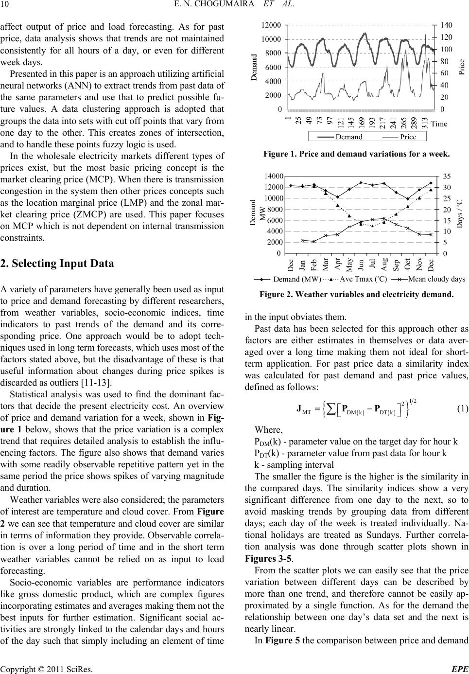

E. N. CHOGUMAIRA ET AL.

affect output of price and load forecasting. As for past

price, data analysis shows that trends are not maintained

consistently for all hours of a day, or even for different

week days.

Presented in this paper is an approach utilizing artificial

neural networks (ANN) to extract trends from past data of

the same parameters and use that to predict possible fu-

ture values. A data clustering approach is adopted that

groups the d ata into sets with cut off po ints that vary from

one day to the other. This creates zones of intersection,

and to handle these point s f uz z y logi c i s used.

In the wholesale electricity markets different types of

prices exist, but the most basic pricing concept is the

market clearing price (MCP). When there is transmission

congestion in the system then other prices concepts such

as the location marginal price (LMP) and the zonal mar-

ket clearing price (ZMCP) are used. This paper focuses

on MCP which is no t dependent on internal tran smission

constraints.

2. Selecting Input Data

A variety of parameters have generally been used as input

to price and demand forecasting by different researchers,

from weather variables, socio-economic indices, time

indicators to past trends of the demand and its corre-

sponding price. One approach would be to adopt tech-

niques used in long term forecasts, which uses most of t he

factors stated above, but the disadvantage of these is that

useful information about changes during price spikes is

discarded as outliers [11-1 3] .

Statistical analysis was used to find the dominant fac-

tors that decide the present electricity cost. An overview

of price and demand variation for a week, shown in Fig-

ure 1 below, shows that the price variation is a complex

trend that requires detailed analysis to establish the influ-

encing factors. The figure also shows that demand varies

with some readily observable repetitive pattern yet in the

same period the price shows spikes of varying magnitude

and duration.

Weather variables were also considered; the parameters

of interest are temperature and cloud cover. From Figure

2 we can see that temperature and cloud cover are similar

in terms of information they provide. Observable correla-

tion is over a long period of time and in the short term

weather variables cannot be relied on as input to load

forecasting.

Socio-economic variables are performance indicators

like gross domestic product, which are complex figures

incorporating e s t im a tes and averages making them not t he

best inputs for further estimation. Significant social ac-

tivities are strongly linked to the calendar days and hours

of the day such that simply including an element of time

Figure 1. Price and demand variations for a week.

Figure 2. Weather variables and electricity demand.

in the input ob viat es t hem.

Past data has been selected for this approach other as

factors are either estimates in themselves or data aver-

aged over a long time making them not ideal for short-

term application. For past price data a similarity index

was calculated for past demand and past price values,

defined as follows:

 





MT DM kDT k









JPP





(1)

Where,

PDM(k) - paramete r val ue on th e t a rget day for ho ur k

PDT(k) - parameter value from past data for hour k

k - sampling interval

The smaller the figure is the higher is the similarity in

the compared days. The similarity indices show a very

significant difference from one day to the next, so to

avoid masking trends by grouping data from different

days; each day of the week is treated individually. Na-

tional holidays are treated as Sundays. Further correla-

tion analysis was done through scatter plots shown in

Figures 3-5.

From the scatter plots we can easily see that the price

variation between different days can be described by

more than one trend, and therefore cannot be easily ap-

proximated by a single function. As for the demand the

relationship between one day’s data set and the next is

nearly linear.

In Figure 5 the comparison between price and demand

E. N. CHOGUMAIRA ET AL.

Figure 3. Correlation between different days for price.

Figure 4. Correlation between different days for demand.

Figure 5. Price ag ai ns t demand.

shows an almost linear relationship up to some point at

which there is a sudden rise in price. This shows that

there is a significant change in the dominant factors that

determine the price at some level of demand, suggesting

that price can be regarded as having multiple trends for

which calculations can be done separately.

Published market data shows the power served, which

is almost always the power demanded. However, infor-

mation about the supplying generators is not readily

available publicly, yet this has more influence on the

price than the magnitude of demand. Normally expensive

generators are dispatched last, so at high demand periods

the price demand ratio tends to be much higher, as can be

seen in Figure 5.

3. System Configuration and Training

3.1. Artificial Neural Networks

An artificial neural network (ANN) is a model that emu-

lates the functional architecture of the human brain. In

this research a multi-layer perceptron ANN is adopted.

This ANN consists of: an input layer, hidden layers and

an output layer as shown in Figure 6. Except for the in-

put layer, each neuron receives a signal that is a linearly

weighted sum of the outputs from all the neurons in the

preceding layer.

Activation of neuron j is then defined as

 





k-1k

ji jii

Ufwu (2)

Where, if neuron j is a hi d den neur on ,

 

1exp

fx x



 







. Otherwise,



xx.

i covers all the neurons in the in the layer (k−1).

Note, the activation of the jth neuron in the kth layer,

uj(k) in (1), is only a function of the activations of the

neurons in the (k−1)th layer and the weights which con-

nect the jth neuron in the kth layer with the neur ons in the

(k−1)th layer. The non-linearity fj(x) can be any mono-

tonic function di fferent i abl e i n t he x domain [14].

3.2. Fuzzy Inference Systems

Fuzzy inference is an implementation of fuzzy logic in

which linguistic like rules map the input onto output

space without strict specification of the input [3,4].

Fuzzy Logic: if X is a universe of discourse with ele-

ments denoted by x, then the fuzzy set A in X is defined

as a set of ordered pairs, A = {x, µA(x)|x ε X}. µA(x) is

called the membership function of x in A. Figure 7 shows

Figure 6. Multi layer perceptron type ANN.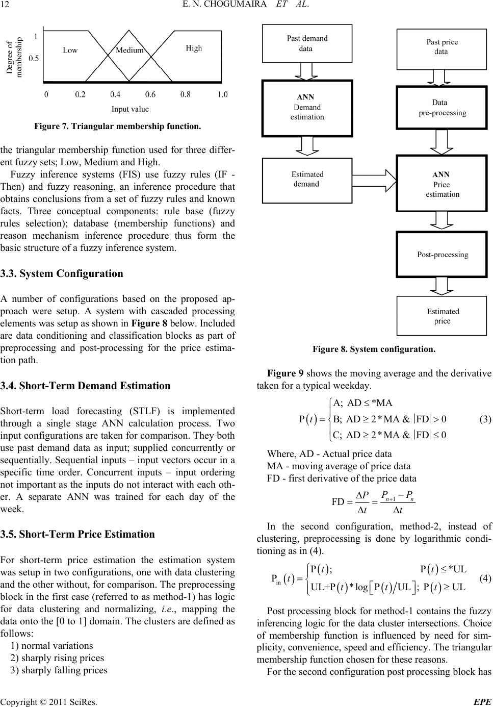

E. N. CHOGUMAIRA ET AL.

Figure 7. Triangular membership function.

the triangular membership function used for three differ-

ent fuzzy sets; Low, Medium and High.

Fuzzy inference systems (FIS) use fuzzy rules (IF -

Then) and fuzzy reasoning, an inference procedure that

obtains conclusions from a set of fuzzy rules and known

facts. Three conceptual components: rule base (fuzzy

rules selection); database (membership functions) and

reason mechanism inference procedure thus form the

basic structure of a fuzzy inference system.

3.3. System Configuration

A number of configurations based on the proposed ap-

proach were setup. A system with cascaded processing

elements was setup as shown in Figure 8 below. Included

are data conditioning and classification blocks as part of

preprocessing and post-processing for the price estima-

tion path.

3.4. Short-Term Demand Estimation

Short-term load forecasting (STLF) is implemented

through a single stage ANN calculation process. Two

input configuration s are taken for comparison. They both

use past demand data as input; supplied concurrently or

sequentially. Sequential in puts – input vectors occur in a

specific time order. Concurrent inputs – input ordering

not important as the inpu ts do not interact with each oth-

er. A separate ANN was trained for each day of the

week.

3.5. Short-Term Price Estimation

For short-term price estimation the estimation system

was setup in two configurations, one with data clustering

and the other without, for comparison. The preprocessing

block in the first case (referred to as method-1) has logic

for data clustering and normalizing, i.e., mapping the

data onto the [0 to 1] domain. Th e clusters are defined as

follows:

1) normal variations

2) sharply rising prices

3) sharply falling prices

Figure 8. System configuration.

Figure 9 shows the movi ng ave rage and the d erivativ e

taken for a typical weekday.



A; AD*MA

PB; AD2*MA & FD

C; AD2*MA & FD0





0











(3)

Where, AD - Actual price data

MA - moving average of price data

FD - first derivative of the price data

FD nn









In the second configuration, method-2, instead of

clustering, preprocessing is done by logarithmic condi-

tioning as in (4).







 





P; P*UL

PUL+P*logPUL; PUL

ttt t













(4)

Post processing block for method-1 contains the fuzzy

inferencing logic for the data cluster intersections. Choice

of membership function is influenced by need for sim-

plicity, convenience, sp eed and efficiency. The triangular

membership function chosen for these reasons.

For the second configuration post processing block has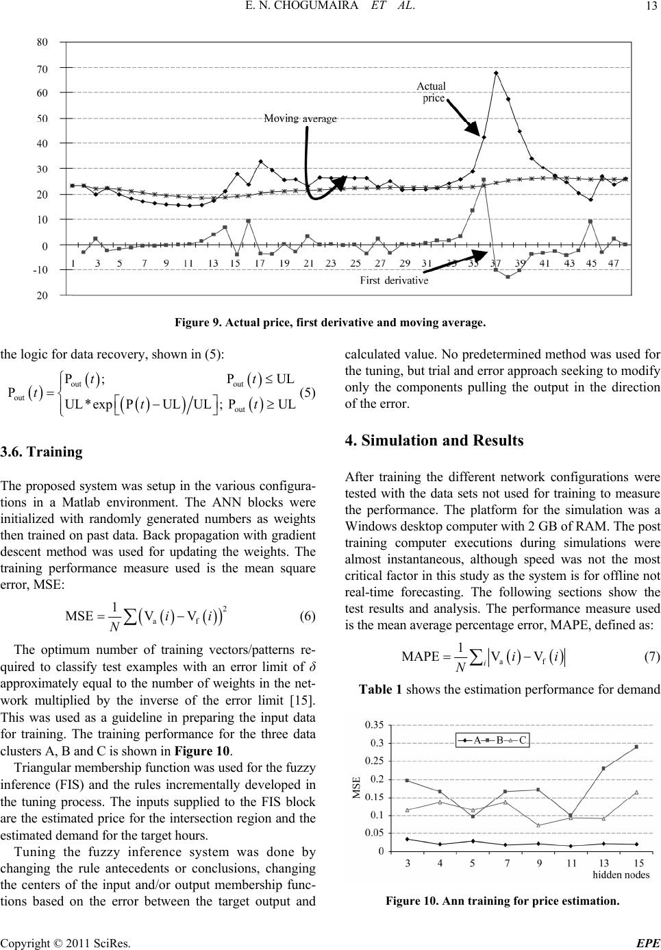

E. N. CHOGUMAIRA ET AL.

Figure 9. Actual price, first derivative and moving average.

the logic for data recovery, shown in (5):

  



out out

out

P; PUL

PUL*expPULUL; PUL













t

(5)

calculated value. No predetermined method was used for

the tuning, but trial and error appro ach seeking to modify

only the components pulling the output in the direction

of the error.

4. Simulation and Results

3.6. Training

After training the different network configurations were

tested with the data sets not used for training to measure

the performance. The platform for the simulation was a

Windows desktop computer with 2 GB of RAM. The post

training computer executions during simulations were

almost instantaneous, although speed was not the most

critical factor in th is study as the system is for o ffline not

real-time forecasting. The following sections show the

test results and analysis. The performance measure used

is the mean average percentage error, MAPE, defined as:

The proposed system was setup in the various configura-

tions in a Matlab environment. The ANN blocks were

initialized with randomly generated numbers as weights

then trained on past data. Back propagatio n with gradient

descent method was used for updating the weights. The

training performance measure used is the mean square

error, MSE:

 



MSEV Vii







(6)

 

MAPEV V





The optimum number of training vectors/patterns re-

quired to classify test examples with an error limit of δ

approximately equal to the number of weights in the net-

work multiplied by the inverse of the error limit [15].

This was used as a guideline in preparing the input data

for training. The training performance for the three data

clusters A, B and C is shown in Figure 10.

i (7)

Table 1 shows the estimation performance for demand

Triangular membership function was used for the fuzzy

inference (FIS) and the rules incrementally developed in

the tuning process. The inputs supplied to the FIS block

are the estimated price for the intersection region and the

estimated demand f or the t ar get hours.

Tuning the fuzzy inference system was done by

changing the rule antecedents or conclusions, changing

the centers of the input and/or output membership func-

tions based on the error between the target output and Figure 10. Ann training for price estimation.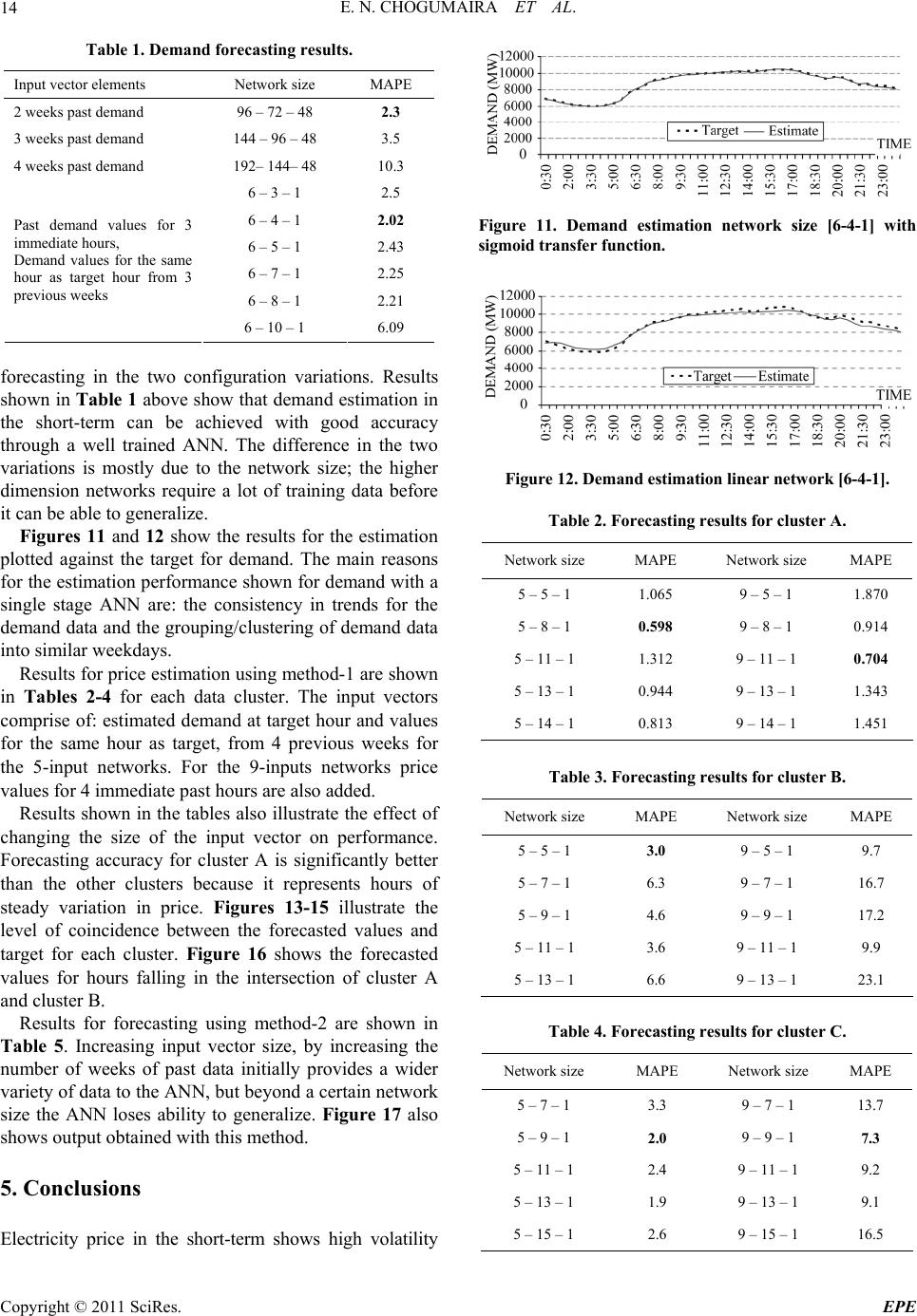

E. N. CHOGUMAIRA ET AL.

Table 1. Demand forecasting results.

Input vector elements Network size MAPE

2 weeks past demand 96 – 72 – 48 2.3

3 weeks past demand 144 – 96 – 48 3.5

4 weeks past demand 192– 144– 48 10.3

6 – 3 – 1 2.5

6 – 4 – 1 2.02

6 – 5 – 1 2.43

6 – 7 – 1 2.25

6 – 8 – 1 2.21

Past demand values for 3

immediate hours,

Demand values for the same

hour as target hour from 3

previous weeks

6 – 10 – 1 6.09

forecasting in the two configuration variations. Results

shown in Table 1 above show that demand estimation in

the short-term can be achieved with good accuracy

through a well trained ANN. The difference in the two

variations is mostly due to the network size; the higher

dimension networks require a lot of training data before

it can be able to generalize.

Figures 11 and 12 show the results for the estimation

plotted against the target for demand. The main reasons

for the estimation performance shown for demand with a

single stage ANN are: the consistency in trends for the

demand data and the grouping /clustering of demand data

into similar weekdays.

Results for price estimation using method-1 are shown

in Tables 2-4 for each data cluster. The input vectors

comprise of: estimated demand at target hour and values

for the same hour as target, from 4 previous weeks for

the 5-input networks. For the 9-inputs networks price

values for 4 immediate past hours are also added.

Results shown in the tables also illustrate th e effect of

changing the size of the input vector on performance.

Forecasting accuracy for cluster A is significantly better

than the other clusters because it represents hours of

steady variation in price. Figures 13-15 illustrate the

level of coincidence between the forecasted values and

target for each cluster. Figure 16 shows the forecasted

values for hours falling in the intersection of cluster A

and cluster B.

Results for forecasting using method-2 are shown in

Table 5. Increasing input vector size, by increasing the

number of weeks of past data initially provides a wider

variety of data to the ANN, but beyond a certain network

size the ANN loses ability to generalize. Figure 17 also

shows output obtained with this method.

5. Conclusions

Electricity price in the short-term shows high volatility

Figure 11. Demand estimation network size [6-4-1] with

sigmoid transfer function.

Figure 12. Demand estimation linear network [6-4-1].

Table 2. Forecasting resu lts for clu ster A.

Network size MAPE Network size MAPE

5 – 5 – 1 1.065 9 – 5 – 1 1.870

5 – 8 – 1 0.598 9 – 8 – 1 0.914

5 – 11 – 1 1.312 9 – 11 – 1 0.704

5 – 13 – 1 0.944 9 – 13 – 1 1.343

5 – 14 – 1 0.813 9 – 14 – 1 1.451

Table 3. Forecasting resu lts for clu ster B.

Network size MAPE Network size MAPE

5 – 5 – 1 3.0 9 – 5 – 1 9.7

5 – 7 – 1 6.3 9 – 7 – 1 16.7

5 – 9 – 1 4.6 9 – 9 – 1 17.2

5 – 11 – 1 3.6 9 – 11 – 1 9.9

5 – 13 – 1 6.6 9 – 13 – 1 23.1

Table 4. Forecasting resu lts for clu ster C.

Network size MAPE Network size MAPE

5 – 7 – 1 3.3 9 – 7 – 1 13.7

5 – 9 – 1 2.0 9 – 9 – 1 7.3

5 – 11 – 1 2.4 9 – 11 – 1 9.2

5 – 13 – 1 1.9 9 – 13 – 1 9.1

5 – 15 – 1 2.6 9 – 15 – 1 16.5

E. N. CHOGUMAIRA ET AL.

Figure 13. Price estimation method-1: cluster A.

Figure 14. Price estimation method-1: cluster B.

Figure 15. Price estimation method-1: cluster C.

Figure 16. Price estimation method-1: intersection AB.

making it difficult to p redict its future value, but with the

proposed approach significant improvement in the fore-

casting performance has been observed. One key element

in the processing is selection of input data and careful

preprocessing. Data clustering into ranges in which ob-

servable trends are maintained allows for th e extraction of

such trends using separate ANN trained for each specific

cluster. Data samples that cannot fit into the strictly de-

fined clusters form intersection zones that, in addition to

ANN, are processed using fuz z y i nference.

Electricity demand shows smoothly varying trends

such that a single stage well tuned ANN blocked man-

aged to achieve good accuracy. Of the two configuration

Table 5. Price forecasting results using method-2.

CaseInput vector elements Network size MAPE

1 Forecasted demand

1 week past price 96 – 72 – 48 18

2 Forecasted demand

2 week past price 144 – 96 – 48 21

3 Forecasted demand

3 week past price 192 – 144 – 488

4 Forecasted demand

4 week past price 240 – 192 – 4817

Figure 17. Price estimation method-2.

options tested comparable performance was obtained.

However, the second configuration that uses large input

vectors comprising of complete days data requires more

computational effort, so the first configuration is consid-

ered optimum.

For electricity price estimation data clustering gives a

comparatively much higher accuracy for the normal price

region and a significantly better result for the times cha-

racterized with spikes. It is therefore concluded that the

way to approach electricity price forecasting while

maintaining all the data is to use a method that employs

data clustering even within a day’s d ata set.

6. References

[1] M. Shahidehpour, H. Yamin and Z. Li, “Market Opera-

tions in Electric Power Systems,” John Wiley & Sons,

Chichester, 2002. doi:10.1002/047122412X

[2] A. K. Topalli, I. Erkmen and I. Topalli, “Intelligent

Short-term Load Forecasting in Turkey,” Electrical Pow-

er and Energy Systems, Vol. 28, 2006, pp. 437-447. doi:

10.1016/j.ijepes.2006.02.004

[3] R. C. Garcia, et al., “GARCH Forecasting Model to Pre-

dict Day-ahead Electricity Prices,” IEEE Transactions on

Power Systems, Vol. 20, No. 2, May 2005, pp. 867-874.

doi:10.1109/TPWRS.2005.846044

[4] M. Stevenson, “Filtering and Forecasting Spot Electricity

Prices in the Increasingly Deregulated Australian Elec-

tricity Market,” Quantitative Finance Research Centre,

University of Technology, Sydney, 2001.

[5] N. Hubele, et al., “Identification of Seasonal Short-term

E. N. CHOGUMAIRA ET AL.

Load Forecasting Models Using Statistical Decision

Functions,” IEEE Transactions on Power Systems, Vol. 5,

No. 1, 1990, pp. 40-5. doi:10.1109/59.49084

[6] M. El-Hawary, et al, “Short-Term Power System Load

Forecasting Using the Iteratively Reweighted Least

Squares Algorithm,” Electrical Power Systems Research,

Vol. 19, 1990, pp. 11-22. doi:10.1016/0378-7796(90)900

03-L

[7] V. S. Kodogiannis and E. M. Anagnostakis, “A Study of

Advanced Learning Algorithms for Short-term Load Fo-

recasting,” Engineering Applications of Artificial Intelli-

gence , Vol. 12, 1999, pp. 159-173. doi:10.1016/S0952-

1976(98)00064-5

[8] G.-C. Liao and T.-P. Tsao, “Application of Fuzzy Neural

Networks and Artificial Intelligence for Short-term load

Forecasting,” Electrical Power Systems Research, Vol.

70, 2004, pp. 237-244. doi:10.1016/j.epsr. 2003.12.012

[9] H. Yamin, M. Shahidehpour and Z. Li, “Adaptive

short-term Price Forecasting using artificial Neural Net-

works in the Restructured Power Markets,” Electrical

Power and Energy Systems, Vol. 26, 2004, pp. 571-581.

doi:10.1016/j.ijepes.2004.04.005

[10] P. Mandal, T. Senjyu, N. Urasaki and T. Funabashi, “A

Neural Network Based Several-Hour-Ahead Electric

Load Forecasting using Similar Days Approach,” Elec-

trical Power and Energy Systems, Vol. 28, 2006, pp.

367-373. doi:10.1016/j.ijepes.2005.12.007

[11] S. Rahman and R. Bhatnager, “An Expert System based

Algorithm for Short Term Load Forecast,” IEEE Trans-

actions on Power Systems, Vol. 3, No. 2, 1988, pp. 392-

399. doi:10.1109/59.192889

[12] Q. Lu, et al., “An Adaptive Nonlinear Predictor with

Orthogonal Escalator Structure for Short-term Load Fo-

recasting,” IEEE Transactions on Power Systems, Vol. 4,

No. 1, 1989, pp. 158-164. doi:10.1109/59.32473

[13] I. Moghram and S. Rahman, “Analysis and Evaluation of

Five Short-Term Load Forecasting Techniques,” IEEE

Transactions on Power Systems, Vol. 4, No. 4, 1989, pp.

1484-1491. doi:10.1109/59.41700

[14] M. Ikeda and T. Hiyama, “ANN Based Designing and

Cost Determination System for Induction Motor,” IEEE

Proceeding Electrical Power Application, Vol. 152, No.

6, 2005, pp. 1595-1602. doi:10.1049/ip-epa:20050173

[15] E. Baum and D. Haussler, “What Net Size Gives Valid

Generalization?” Neural Computation, Vol. 1, No. 1,

1989, pp. 151-160. doi:10.1162/neco.1989.1.1.151