Predictability of Al-Mn Alloy Exposure Time Based on Its As-Cast Weight and Corrosion Rate in Sea Water Environment

doi:10.4236/jmmce.2013.16046

Paper Menu >>

Journal Menu >>

Journal of Minerals and Materials Characterization and Engineering, 2013, 1, 307-314

Published Online November 2013 (http://www.scirp.org/journal/jmmce)

http://dx.doi.org/10.4236/jmmce.2013.16046

Open Access JMMCE

Predictability of Al-Mn Alloy Exposur e Time Based on Its

As-Cast Weight and Corrosion Rate in Sea Water

Environment

Chukwuka Nwoye1*, Simeon Neife2, Ebere Ameh3, Awo Nwobasi4, Ndubuisi Idenyi5

1Department of Metallurgical and Materials Engineering, Nnamdi Azikiwe University, Awka, Nigeria

2Department of Metallurgical and Materials Engineering, University of Nigeria, Nsukka, Nigeria

3Department of Metallurgical and Materials Engineering, Enugu State University of Science & Technology, Enugu, Nigeria

4Department of Technology and Vocational Education, Ebonyi State University, Abakiliki, Nigeria

5Department of Industrial Physics, Ebonyi State University, Abakaliki, Nigeria

Email: *[email protected]

Received September 8, 2013; revised October 18, 2013; accepted October 30, 2013

cense, which permits unrestricted use, distribution, and reproduction in any medium, provided the original work is properly cited.

ABSTRACT

This paper presents the predictability of aluminium-manganese alloy exposure time based on its as-cast weight and

corrosion rate in sea water environment. The validity of the derived model: 26.67 0.550.29







 is rooted on the

core expression: 0.03750.0206 0.0109





 where both sides of the expression are correspondingly approximately

equal. Statistical analysis of model-predicted and experimentally evaluated exposure time for each value of as-cast

weight and alloy corrosion rate considered shows a standard error of 0.0017% & 0.0044% and 0.0140% & 0.0150%

respectively. The depths of corrosion penetration (at increasing corrosion rate: 0.0104 - 0.0157 mm/yr) as predicted by

derived model and obtained from experiment are 0.7208 × 10−4 & 1.0123 × 10−4 mm and 2.5460 × 10−4 & 1.8240 × 10−4

mm (at decreasing corrosion rate: 0.0157 - 0.0062 mm/yr) respectively. Deviational analysis indicates that the maxi-

mum deviation of the model-predicted alloy exposure time from the corresponding experimental value is less than 10%.

Keywords: Prediction; Exposure Time; Al-Mn Alloys; Sea Water; Alloy As-Cast Weight; Corrosion Rate

1. Introduction

The service performance of metals (or alloy), irrespective

of the exposure environment is largely affected by their

physical and mechanical properties such as hardness,

weldability, toughness, malleability, ductility, resistance

to fatique etc. It is therefore vital to consider these and

other basic properties of metals or alloys when proposing

their application for fabrication and other engineering

purposes.

Researchers [1] have suggested the need to know the

specific corrosion rates of different metals and alloys in

different application environment in order to know the

materials that can withstand outdoor structural applica-

tions.

The stability of metals or alloys in an aggressive envi-

ronment has been reported [2] to basically depend on the

protective properties of organic or inorganic films as well

as on the layer of corrosion products. The scientists con-

cluded that the ability of films to act as controlling barri-

ers against different kinds of corrosion attack is depend-

ent on film properties such as chemical composition,

adhesion, conductivity, solubility, morphology and hy-

groscopicity. Several researchers [1,3] reported that the

highlighted characteristic of films in turn depends on

environmental variables such as atmospheric conditions,

type and amount of pollutants as well as wet-dry cycle,

the chemical composition and metallurgical history of the

metals or alloys and physicochemical properties of coat-

ing.

Malfunctioning of engineering structures and equip-

ment due to corrosion has been reported [4] to stem from

tragic carelessness in plumbing, equipment manufacture

and installation, with possibility of explosion, fire and

spread of toxic materials in living environment. This is

accompanied by some costs such as replacement of cor-

roded equipment, disturbance in processes due to equip-

*Corresponding author.

C. NWOYE ET AL.

308

ment corrosion, shutdown of plants due to replacement of

corroded equipment, impurity in processed products due

to corrosion as well as waste of the products of those

vessels which are attacked by corrosion. The report indi-

cates that about 70 percent of losses can be prevented by

observing related principles and instructions.

One of the main problems in oil and gas industries is

corrosion of pipelines and other engineering structures.

This has always resulted in huge economic setback due

to large sum of money spent in trying to combat it. Based

on the forgoing, there is a great need to develop engi-

neering materials that are corrosion resistant to avoid

abrupt failure of the engineering structures.

Recently, the corrosion characteristics of selected fer-

rous metal samples (plain and alloyed ductile iron, low

carbon steel and austenitic stainless steel) in crude oil

were investigated by using weight loss method [5]. Stud-

ies carried out during this work show that all the materi-

als experience gain in weight within the first 10 days in

the medium. This weight gain is attributed to the forma-

tion of hard and passive phases which acted as strong

protective barriers to corrosion. It was also observed that

the rate of corrosion decreased with increase in the num-

ber of days of exposure for all the coupons, this may be

probably due to the deposition of corrosion products that

tend to shield the corroding surface from further corro-

sion attack, thereby depressing the rate of corrosion. This

result shows that despite of initial low corrosion resis-

tance of plain ductile iron, it can still be considered,

alongside other materials, for application in pipelines and

storage facilities for crude oil.

Studies [6] on the corrosion behaviour of carbon steel

under natural and stagnant seawater conditions have

showed that the alloy is more corrosive in anaerobic stag-

nant sea-water conditions than that in aerobic conditions.

The study also revealed that in both aerobic and anaero-

bic exposures, corrosion was more aggressive on hori-

zontally oriented coupons compared to vertically orient-

ed samples.

The corrosion behaviour of low carbon steel has also

been investigated [7] in natural seawater and various

synthetic seawaters. It was found that the steel corroded

nearly four times faster in a 3.5% NaCl solution than in

natural seawater for an exposure time of 21 days. The

corrosion rate after immersion in synthetic seawaters was

found to be similar to the corrosion rate after immersion

in natural seawater. Calcium carbonate (aragonite) de-

posits were found on the surface of the steel after immer-

sion in natural seawater and the synthetic seawaters.

Some magnesium-containing deposits were also found

after immersion in the natural seawater. These deposits

act as a barrier against oxygen diffusion and thereby

lower the corrosion rate. The morphology of the calcium

carbonate deposits that formed during immersion in the

natural seawater was found to be different from those

formed during immersion in the solution.

It has been shown [8] that MnAl6 formed from Al and

Mn has almost the same electrode potential as aluminium

and this compound is capable of dissolving iron which

reduces the detrimental effect of Mn. Commercial Al-Mn

alloys contains up to 1.25% manganese although the

maximum solid solubility of this element in aluminium is

as high as 1.82%. This limitation was imposed because

the presence of iron as impurity reduces the solubility

and there is a danger that large primary particles of

MnAl6 will form with a disastrous effect on local ductil-

ity.

Polmear [8] reported that Al-Mn alloys belong to the

3xxx series of alloys which are used for the manufacture

of roofing sheets. These sheets are subject to corrosion

because of the presence of moisture and oxygen in the

atmosphere. The corrosion of this alloy is due to the

strong affinity aluminium has for oxygen which results to

its oxidation and subsequent formation of oxide film.

Ekuma et al. [9] reported that with time, this film be-

comes passive to further oxidation and stable in aqueous

media when the pH is between 4.0 and 8.5. It is impor-

tant to state that the passive films can break and fall off,

hence exposing the surface of the alloy to further corro-

sion.

Studies [4] on corrosion management indicate that it

offers preventive strategies in two technical and non-

technical domains. Technical domains as preventive

strategies are highly important. These includes: 1) Up-

grading planning methods and using advanced planning

ones to better corrosion management and so prevent

avoidable corrosion costs. In this vein, planning methods

must change and the best corrosion technologies must be

available for planners. 2) Improving corrosion technolo-

gies via research and development. Corrosion can be

controlled in most industries by using scientific methods

and new technological achievements.

Non-technical domain as preventive strategies includes:

1) Enhancing the employees' awareness about the high

costs of corrosion and saving costs result in correct ap-

plication of existing technologies and corrosion costs.

Thus a lot of corrosion problems are due to lack of

awareness about corrosion management and accountabil-

ity of people in exchanging operations, inspection and

maintenance of management system. 2) Changing guide-

lines, protocols, standards and management methods to

reduce corrosion costs by correct corrosion management,

resulting in effective control of corrosion and safe opera-

tion and increase in shelf life of equipment. 3) Amend-

ing and generalization of employees’ instruction to in-

troduce and identify corrosion control. 4) Changing and

amending wrong belief about not being able to do any-

thing about corrosion and making new decisions in pre-

Open Access JMMCE

C. NWOYE ET AL. 309

venting this phenomenon.

The aim of this work is to ascertain the predictability

of aluminium-manganese alloy exposure time based on

its as-cast weight and corrosion rate in sea water envi-

ronment. The model to be derived is expected to evaluate

and predict directly the exact time (exposure time) at

which the Al-Mn alloy should be exposed in the sea wa-

ter environment putting into consideration its as-cast

weight (alloy initial weight before corrosion) and corro-

sion rate in such environment. The essence of this work

is to determine the exact exposure time for a weighed

Al-Mn alloy whose corrosion rate in the sea water envi-

ronment is already known. This rules out exposure of the

alloy to the corrosive environment longer than necessary;

a situation that could result to very disastrous, undue

corrosion penetration on the alloy and invariably, failure.

The success of this work would eventually reduce abrupt

failure of Al-Mn alloy in sea water environment due to

over exposure.

2. Materials and Methods

Materials used for this work are aluminium of 96% pu-

rity and pure granulated manganese. Details of the ex-

perimental procedure and associated process conditions

are as stated in the previous report [10].

2.1. Model Formulation

Experimental data obtained from research work [10]

were used for this work. Computational analysis of the

experimental data [10] shown in Table 1, gave rise to

Table 2 which indicate that:





 (1)

Introducing the values of K, S and Ne into Equation (1)

reduces it to:

0.03750.0206 0.0109





 (2)

0.0206 0.0109

0.0375



















(3)

26.67 0.550.29





 (4)

where K = 0.0375; Overall Al-Mn alloy-sea water tem-

perature interaction factor (determined using C-NIK-

BRAN [11]). S = 0.0206; First order alloy degradability

Table 1. Variation of corrosion rate with exposure time and

alloy as-cast weight [10].

(β) (mm/yr) (α) (hrs) (γ) (g)

0.0104

0.0140

0.0157

0.0105

0.0062

336

450

504

600

672

12.0754

12.3911

12.4775

13.2012

13.7434

Table 2. Variation of 0.0375α with γ + 0.0206β – 0.0109.

0.0375α(γ) 0.0206β0.0109 γ + 0.0206β – 0.0109

0.00144

0.00193

0.00216

0.00257

0.00288

0.0104

0.0140

0.0157

0.0105

0.0062

0.00021

0.00029

0.00032

0.00022

0.00013

0.0109

0.00141

0.00179

0.00192

0.00252

0.00293

Coefficient (determined using C-NIKBRAN [11]); N

0.0109; Film solubility-adhesion ratio in sea water (de-

termined using C-NIKBRAN [11]); (β)= Corrosion rate

(mm/yr); (α) = Exposure time (yr); (γ) = Initial weight of

alloy (kg).

2.2. Boundary and Initial Conditions

Consider solid Al-Mn alloy exposed to sea water envi-

ronment and interacting with some corrosion-induced

agents. The sea water is assumed to be affected by un-

wanted dissolved gases. Range of exposed time consid-

ered: 0.0384 - 0.0767 yrs (336 - 672 hrs). Initial weight

range considered: 0.0121 - 0.0137 kg (12.0754 - 13.7434 g).

Purity of aluminium used: 96%. Concentration of

manganese addition: 4%. Details of experiment and other

process conditions are as stated in the experimental tech-

nique [10].

The boundary conditions are: aerobic environment to

enhance Al-Mn alloy oxidation (since the sea water con-

tains oxygen). At the bottom of the exposed alloy, a zero

gradient for the gas scalar are assumed. The exposed

alloy is stationary. The sides of the solid are taken to be

symmetries.

3. Results and Discussions

The derived model is Equation (4). Computational analy-

sis of Table 1 gave rise to Tables 2 and 3. The derived

model is two-factorial in nature because it is a constituent

of two input process factors: as-cast weight (initial alloy

weight) and corrosion rate. This implies that the pre-

dicted exposure time for the Al-Mn alloy in sea water

environment is dependent on just two factors: as-cast

weight and corrosion rate of the alloy.

3.1. Model Validation

The validity of the model is strongly rooted on Equation

(2) (core model equation) where both sides of the equa-

tion are correspondingly approximately equal. Table 2

also agrees with Equation (2) following the values of

0.0375α and γ + 0.0206β – 0.0109 evaluated from the

experimental results in Table 1 . Furthermore, the derived

model was validated by comparing the exposure time

predicted by the model and that obtained from the ex-

periment [10]. This was done using various analytical

techniques.

Open Access JMMCE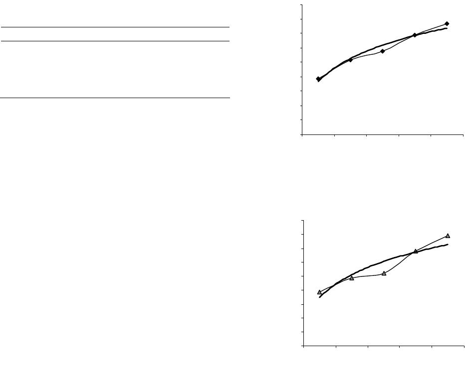

C. NWOYE ET AL.

310

Table 3. Evaluated variation of corrosion rate of Al-Mn

alloy with its as-cast weight and exposure time.

(β) (mm/yr) (α) (yrs) (γ) (kg)

0.0104

0.0140

0.0157

0.0105

0.0062

0.0384

0.0514

0.0575

0.0685

0.0767

0.0121

0.0124

0.0125

0.0132

0.0137

3.2. Computational Analysis

Computational analysis of the experimental and model-

predicted exposure time was carried out to ascertain the

degree of validity of the derived model. This was done

by comparing the depth of corrosion penetration obtained

by calculations involving experimental results, and pre-

dicted directly by the model.

The depth of corrosion penetration for Al-Mn alloy

during the period of exposure in the sea water environ-

ment CD (mm) was calculated from the equation;





  (5)

Δβ = Change in the corrosion rates β2, β1 within a range

of exposure time: α1 - α2. Δα = Change in the alloy ex-

posure time α2, α1.

Considering experimental results of points (0.0384,

0.0104) and (0.0575, 0.0157) for (

) and (

)

respectively

(during the period corrosion rate was in-

creasing)

, (as in

Figure 1

) and substituting them into

Equation (5), gives 1.0123 × 10

−

mm as the depth of

corrosion penetration on the alloy

during the actual cor-

rosion process

Also similar plot (as in

Figure 2

) using

model-predicted results of points (0.0384, 0.0104) and

(0.0520, 0.0157) for (

) and (

) respectively,

during the period corrosion rate was increasing

and sub-

stituting them into Equation (5) gives the depth of

cor-

rosion penetration on the alloy as

0.7208 × 10

−

mm.

This is the model-predicted depth of

corrosion penetra-

tion on the alloy. Furthermore,

substituting experimental

results of points (0.0575, 0.0157) and (0.0767, 0.0062)

for (

) and (

) respectively

(during the period

corrosion rate was decreasing)

, (as in

Figure 1

) into

Equation (5), gives

−1.8240

10−4

mm as the depth of

corrosion penetration on the alloy.

On other hand, substituting

model-predicted results of

points (0.0520, 0.0157) and (0.0788, 0.0062) for (

)

and (

) respectively,

during decreasing corrosion

rate

(as in

Figure 2

) into Equation (5) gives

−2.5460

10−4 mm. The negative signs preceding the magnitudes

of the depth of corrosion penetration do not indicate that

the depth of the penetration is negative, but that the cor-

rosion penetration occurred when the alloy corrosion rate

is decreasing and so are discarded. Based on the forego-

ing, the depths of corrosion penetration during the period

corrosion rate was decreasing as obtained from experiments

= 0.9627

0.01

0.02

0.03

0.04

0.05

0.06

0.07

0.08

0.09

0.01040.0140.0157 0.0105 0.0062

Corrosion rate (mm/yr)

Exposure time (yr)

Figure 1. Coefficient of determination between alloy expo-

sure time and its corrosion rate as obtained from the ex-

periment [10].

= 0.8722

0.01

0.02

0.03

0.04

0.05

0.06

0.07

0.08

0.09

0.01040.0140.0157 0.01050.0062

Corrosion rate (mm/ yr)

Exposure time (yr)

Figure 2. Coefficient of determination between alloy expo-

sure time and its corrosion rate as predicted by derived

model.

[10] and derived model are 1.8240

10−4

and

2.5460

10−4 mm respectively.

3.3. Statistical Analysis

Statistical analysis of model-predicted and experimen-

tally evaluated exposure time for each value of as-cast

weight and alloy corrosion rate considered shows a stan-

dard error (STEYX) of 0.0017% & 0.0044% and

0.0140%

& 0.0150

% respectively. The standard error was evalu-

ated using a Microsoft Excel [12].

Furthermore, as a way validating the derived model,

regression model (highlighted from [12]) was used to

predict the corresponding exposure time for the values of

as-cast weight and corrosion rate considered, and the

results are shown in Figures 3 and 4. On the other hand,

the standard error in predicting the exposure time for

each value of corrosion rate considered is 0.0119%.

The correlations between exposure time and as-cast

Open Access JMMCE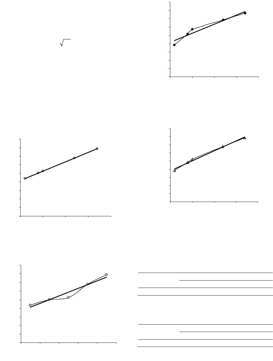

C. NWOYE ET AL. 311

weight as well as exposure time and corrosion rate as

obtained from derived model, regression model and ex-

perimental results [10] were calculated. This was done by

considering the coefficients of determination R2 from

Figures 1-6, using the equation:

RR (6)

The evaluated correlations are shown in Tables 4 and

5. The model was also validated by comparing its results

of evaluated correlations between exposure time and as-

cast weight as well as exposure time and corrosion rate

with that evaluated using experimental and regression

model-predicted results. Tables 4 and 5 show that the

correlation results from experiment, derived model (D-

MoD) and R-MoD are in proximate agreement.

3.4. Graphical Analysis

Results predicted by the regression model were plotted;

= 1

0.01

0.02

0.03

0.04

0.05

0.06

0.07

0.08

0.09

0.012 0.0125 0.013 0.0135 0.014

As-cast weight (kg)

Exposure time (yr)

Figure 3. Coefficient of determination between alloy expo-

sure time and its as-cast weight as predicted by regression

model.

= 0.9368

0.01

0.02

0.03

0.04

0.05

0.06

0.07

0.08

0.09

0.01040.0140.0157 0.0105 0.0062

Corrosion rate

(

mm/

)

Exposure time (yr)

Figure 4. Coefficient of determination between alloy expo-

sure time and its corrosion rate as predicted by regression

= 0.933

0.01

0.02

0.03

0.04

0.05

0.06

0.07

0.08

0.09

0.0120.0125 0.0130.0135 0.01

As-cast wei

(

Exposure time (yr)

Figure 5. Coefficient of determination between alloy expo-

sure time and its as-cast weight as obtained from the ex-

periment [10].

= 0.9918

0.01

0.02

0.03

0.04

0.05

0.06

0.07

0.08

0.09

0.012 0.0125 0.0130.0135 0.014

As-cast weight (kg)

Exposure time (yr)

Figure 6. Coefficient of determination between alloy expo-

able 4. Comparison of the correlations between exposure

sure time and its as-cast weight as predicted by derived

model.

time and alloy as-cast weight as evaluated from experimen-

tal, derived model and re gre ssion pr e dic te d results.

Based on alloy as-cast weight

Analysis ExoD

D D-MoD

R-M

CORRELL 0 .96590.9659 1.0000

able 5. Comparison of the correlations between exposure T

time and alloy corrosion rate as evaluated from experimen-

tal, derived model and re gre ssion pr e dic te d results.

Based on corrosion rate

Analysis ExD D-MoD R-MoD

CORRELL 0 .98120.9339 0.9679

xposure time against alloy as-cast weight and corrosion e

rate respectively along with results from the experiment

and derived model to analyze its spread and trend relative

to results from experiment and derived model.

model.

Open Access JMMCE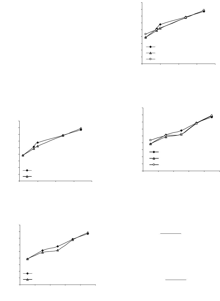

C. NWOYE ET AL.

312

Comparative graphical analysis of Figures 7 and 8

3.5. Deviational Analysis

sure time from the experi-

shows very close alignment of the curves from derived

model and experiment. Figures 9 and 10 also indicate a

close alignment of curves from derived model (MoD),

regression model (R-MoD) predicted results as well as

experimental (ExD).

Comparative analysis of expo

ment [10] and derived model revealed deviations on the

part of the model-predicted values relative to values ob-

tained from the experiment. This is attributed to the fact

that the surface properties of the alloy and the physio-

chemical interaction between the alloy and corrosion

induced agents (in the sea water) were not considered

during the model formulation. This necessitated the in-

troduction of correction factor, to bring the model-pre-

dicted corrosion rate to those of the corresponding ex-

perimental values.

0.01

0.02

0.03

0.04

0.05

0.06

0.07

0.08

0.09

0.0120.0125 0.0130.0135 0.014

As-cast weight (kg)

Exposu re time (yr)

ExD

MoD

Figure 7. Comparison of the alloy exposure time (relative to

its as-cast weight) as obtained from experiment [10] and

derived model.

0.01

0.02

0.03

0.04

0.05

0.06

0.07

0.08

0.09

0.01040.0140.0157 0.0105 0.0062

Corrosion rate

(

mm/

)

Exposed time (yr)

ExD

MoD

Figure 8. Comparison of the alloy exposure time (relative to

derived model.

its corrosion rate) as obtained from experiment [10] and

0.01

0.02

0.03

0.04

0.05

0.06

0.07

0.08

0.09

0.012 0.0125 0.0130.0135 0.014

As-cast weight (kg)

Exposure time (yr)

ExD

MoD

ReG

Figure 9. Comparison of the alloy exposure time (relative to

its as-cast weight) as obtained from experiment [10] derived

and regression model.

0.01

0.02

0.03

0.04

0.05

0.06

0.07

0.08

0.09

Exp osure time (yr)

ExD

MoD

0.0104 0.014 0.01570.01050.0062

Corrsion rate

(

mm/

)

ReG

Figure 10. Comparison of the alloy exposure time (relative

to its corrosion rate) as obtained from experiment [10] de-

predicted corrosion rate from

at of

rived and regression model.

Deviation (Dn) of model-

th the experiment[10] is given by

–100

CR CR

Dn 







(14)

Correction factor (Cr) is the negative

i.e.

of the deviation

Cr Dn



 (15)

therefore

–100

CR CR

Cr E



 





(16)

where: PCR = Model-predicted exposure ti

y the corre-

me (yr); ECR =

Exposure time obtained from experiment [10] (yr); Cr =

Correction factor (%); Dn = Deviation (%).

Introduction of the corresponding values of Cr from

Equation (9) into the model gives exactl

Open Access JMMCE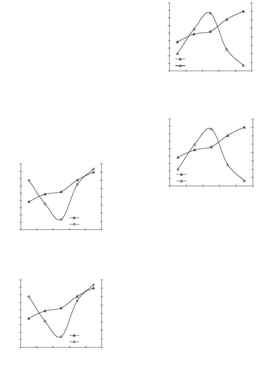

C. NWOYE ET AL. 313

the corre-

of the curve in Figures 13 and 14 is op-

onding experimental corrosion rate.

Figures 11 and 12 show that the maximum deviation

of the mode-predicted exposure time from

onding experimental values is less than 10% and quite

within the acceptable deviation limit of experimental

results. These figures show that least and highest magni-

tudes of deviation of the model-predicted exposure time

(from the corresponding experimental values) are 0% and

−9.57% which corresponds to exposure times: 0.0384

and 0.0520 yr, alloy as-cast weight; 0.0121 and 0.0125

kg and alloy corrosion rates; 0.0104 and 0.0157 mm/yr

respectively.

Comparative analysis of Figures 11-14 indicates that

the orientation

site that of the deviation of model-predicted exposure

time (Figures 11 and 12). This is because correction

factor is the negative of the deviation as shown in Equa-

tions (8) and (19). It is believed that the correction factor

takes care of the effects of the surface properties of the

alloy which were not considered during the model for-

mulation. Figures 13 and 14 indicate that the least and

highest magnitudes of correction factor to the model-

0.01

0.02

0.03

0.04

0.05

0.06

0.07

0.08

0.09 4

0.0121 0.0124 0.0125 0.0132 0.0137

As-cast weight (kg)

Exposure tim e (yr)

-12

-10

-8

-6

-4

-2

Devia tion (%)

Expo time

Deviation

Figure 11. Variation of model-predicted alloy exposure time

(relative to its as-cast weight) with its associated devi ation

from experimental values.

0.01

0.02

0.03

0.04

0.05

0.06

0.07

0.08

0.09

0.01040.0140.0157 0.0105 0.0062

Co rrosion rate

(

mm/

)

Exposure time (yr)

-12

-10

-8

-6

-4

-2

Deviation (%)

Expo time

Deviation

Figure 12. Variation of model-predicted alloy exposure time

(relative to its corrosion rate) with its associated devi

from experimental values. ation

0.01

0.02

0.03

0.04

0.05

0.06

0.07

0.08

0.09

Exposure time (yr

-4

-2

Correction factor (%)

)

Expo time

0.01210.0124 0.0125 0.01320.0137

As-cast wei

(

Corr.factor

Figure 13. Variation of model-predicted alloy exposure time

(relative to its as-cast weight) with its associated correion

factor. ct

0.01

0.02

0.03

0.04

0.05

0.06

0.07

0.08

0.09 12

0.0104 0.014 0.01570.01050.0062

Corrosion rate (mm/yr)

Exposure time (yr)

-4

-2

Correction f actor (% )

Expo time

Corr.factor

Figure 14. Variation of model-predicted alloy exposure time

(relative to its corrosion rate) with its associated correion

factor.

to exposure times: 0.0384 and 0.0520 yr, alloy

Aluminium-manganese alloy exposure time was evalu-

based on its as-cast weight and cor-

predicted exposure time are 0 and +9.57% which corre-

sponds

as-cast weight; 0.0121 and 0.0125 kg and alloy corrosion

rates; 0.0104 and 0.0157 mm/yr respectively.

It is important to state that the deviation of model pre-

dicted results from that of the experiment is just the

magnitude of the value. The associated sign preceding

the value signifies that the deviation is deficit (negative

sign) or surplus (positive sign).

4. Conclusion

ated and predicted

rosion rate in sea water environment. The validity of the

derived model was rooted on the core expression:

0.03750.0206 0.0109







 where both sides of

the expression are correspondingly approximately equal.

Statistical analysis of model-predicted and experimen-

tally evaluated exposure time for each value of as-cast

weight and alloy corrosion rate considered shows a stan-

dard error of 0.0017% & 0.0044% and

0.0140% &

Open Access JMMCE

C. NWOYE ET AL.

Open Access JMMCE

314

[1] C. E. Ekuma and N. E. Idenyi, “Statistical Analysis of the

Influence of tion of Corrosion

from Its Param of Physics, Vol. 1,

0.0150

% respectively. The depths of corrosion penetra-

tion (at increasing corrosion rate: 0.0104 - 0.0157 mm/yr)

as predicted by derived model and obtained from ex-

periment are

0.7208 × 10

−

& 1.0123 × 10

−

mm and

2.5460

10−4 & 1.8240

10−4

(at decreasing corro-

sion rate: 0.0157 - 0.0062 mm/yr) respectively. Devi-

ational analysis indicates that the maximum deviation of

the model-predicted alloy exposure time from the corre-

sponding experimental value is less than 10%.

REFERENCES

Environment on Predic

eters,” Research Journal

No. 1, 2007, pp. 27-34.

http://dx.doi.org/10.3923/rjp.2007.27.34

[2] M. Stratmann, K. Bohnenkamp and W. J. Engell, “An

Electrochemical Study of

ers,” Corrosion Science, Vol. 23, 1983, pp

Phase Transitions in Rust Lay

. 969-985.

ci-

[3] S. G. Stratmann and H. Strekcel, “On the Atmospheric

Corrosion of Metals Which Are Covered with Thin Elec-

trolyte Layers II, Experimental Results,” Corrosion S

ence, Vol. 30, No. 6-7, 1990, pp. 697-714.

http://dx.doi.org/10.1016/0010-938X(90)90033-2

[4] A. Samim, and S. Zarinabadi, “An Analysis of Polyeth-

ylene Coating Corrosion in Oil and Ga

Journal of American Science, Vol. 7, 2011, pp

s Pipelines,”

. 1032-

. Borode, S. O. O. Olusunle and O. O. Adewoye,

da, “An Evaluation of Carbon Steel Corro-

n Steel in Natural and

n, 1981.

e Corrosion Susceptibility of Alu-

1036.

[5] O. Ogundare, I. M. Momoh, O. J. Akinribide, A. R. Ade-

tunji, J. O

“Comparative Study of Corrosion Sensitivity of Selected

Ferrous Metals in Crude Oil,” Journal of Minerals &

Materials Characterization & Engineering, Vol. 11, 2012,

pp. 559-568.

[6] S. L. Jason, I. R. Richard, J. L. Edward, U. F. Alexander

and J. L. Bren

sion under Stagnant Seawater Conditions,” Biofouling:

The Journal of Bioadhesion and Biofilm Research, Vol.

20, No. 4-5, 2004, pp. 237-247.

[7] H. Möller, E. T. Boshoff and H. Froneman, “The Corro-

sion Behaviour of a Low Carbo

Synthetic Seawaters,” The Journal of the South African

Institute of Mining and Metallurgy, Vol. 106, 2006, pp.

585-592.

[8] I. J. Polmear, “Light Alloys,” Edward Arnold Publishers

Ltd., Londo

[9] C. E. Ekuma, N. E. Idenyi and A. E. Umahi, “The Effects

of Zinc Addition on th

minium Alloys in Various Tetraoxosulphate (vi) Acid

Environments,” Journal of Applied Science, Vol. 7, No. 2,

2007, pp. 237-241.

http://dx.doi.org/10.3923/jas.2007.237.241

[10] N. E. Idenyi, S. P. I. Ogah

Behaviour of Al-Mn Binary Alloy System

and J. C. Mbazor, “Corrosion

s in Selected

Environments,” Journal of Metallurgical and Materials

Engineering, Vol. 5, 2010, pp. 37-42.

[11] C. I. Nwoye, “C-NIKBRAN-Data Analytical Memory

(Software),” 2008.

[12] Microsoft Excel, 2003 Version.