Experimental and Numerical Evaluation and Optimization of a Non Standard Pitot/Sampling Probe

doi:10.4236/eng.2013.512118

Paper Menu >>

Journal Menu >>

Engineering, 2013, 5, 967-974

Published Online December 2013 (http://www.scirp.org/journal/eng)

http://dx.doi.org/10.4236/eng.2013.512118

Open Access ENG

Experimental and Numerical Evaluation and Optimization

of a Non Standard Pitot/Sampling Probe

Andrea Shmueli1, Tor Erling Unander2, Ole Jørgen Nydal1

1Norwegian University of Science and Technology, Department of Energy and Process Engineering, Trondheim, Norway

2Department of Petroleum Research, SINTEF, Trondheim, Norway

Email: [email protected]

Received September 4, 2013; revised October 4, 2013; accepted October 11, 2013

which permits unrestricted use, distribution, and reproduction in any medium, provided the original work is properly cited.

ABSTRACT

An isokinetic sampling probe is designed and constructed to measure entrained liquid droplet fluxes in separated gas-

liquid pipe flows. This probe also has the capability of working as a non-standard Pitot tube when the sampling is

stopped. CFD simulations using the commercial software Ansys CFX were carried out for single phase gas flow to

analyze the non-standard design. Pitot tube velocity calculations and isokinetic sampling conditions were studied. The

predicted results were compared against theoretical velocity profiles from the literature and with gas single phase ex-

perimental data acquired in a horizontal 49 m long steel pipeline with an internal diameter of 69 mm. The experiments

were done by using a dense gas (SF6) at 7 bara. An asymmetry of the experimental velocity profiles reproduced with

the numerical simulations. The CFD simulations made it possible to verify the design and predict and correct an instal-

lation problem.

Keywords: Isokinetic Probe; Pitot Tube; CFD; Flow; Installation Effects

1. Introduction

Pitot probes are devices which are commonly used in the

industry to measure the local velocity in gases flowing in

pipes or ducts. The dynamic pressure





dts

PPP of

the fluid stream is measured by the Pitot probe and the

velocity can be calculated from it. When the gas com-

pressibility effect can be neglected, the local velocity can

be calculated from:





 (1)

where C is a calibration constant.

The Pitot tubes have been used for measuring the gas

dynamic pressure in gas-liquid flows [1-4]. However, the

calculation of the velocity from the pressure values is not

straightforward and will depend upon the flow regime

[5]. In gas flow with liquid droplet entrainment, it is a

common practice to use isokinetic sampling probes to

extract flow from the main stream in order to get the lo-

cal dispersed droplet flux. These probes are designed to

have a Pitot-like geometry and pressure tapings and can

be designed to measure the local velocity when the sam-

pling is stopped. The probes are generally not standard so

their design must be tested and validated. Two aspects

that should be taken into account when designing a new

Pitot probe are the velocity measured by the Pitot probe

in an ideal flow and the effect of the probe presence on

the upstream flow [6]. Due to the complexity of multi-

phase flows, the probe design and installation are evalu-

ated by using single phase gas conditions.

In this paper, a design and installation assessment of

the non standard Pitot/sampling probe is done by the

analysis of single phase gas experimental data and simu-

lation of the probe current design using CFD tools.

2. Probe Design

The sampling/Pitot probe is designed to be able to sam-

ple a liquid flux. Some authors have demonstrated that

the effect of the sampling tube diameter and length of the

probe on the measured droplet flux is negligible [7,8].

However in this study the criteria used to select the probe

diameter was associated with the maximum possible

droplet size. Two correlations were used: one for gas/

liquid systems and another one for liquid/liquid systems.

Kocamustafaogullari et al. (1994) [9 ] presented a corre-

lation for the maximum droplet diameter in annular flows.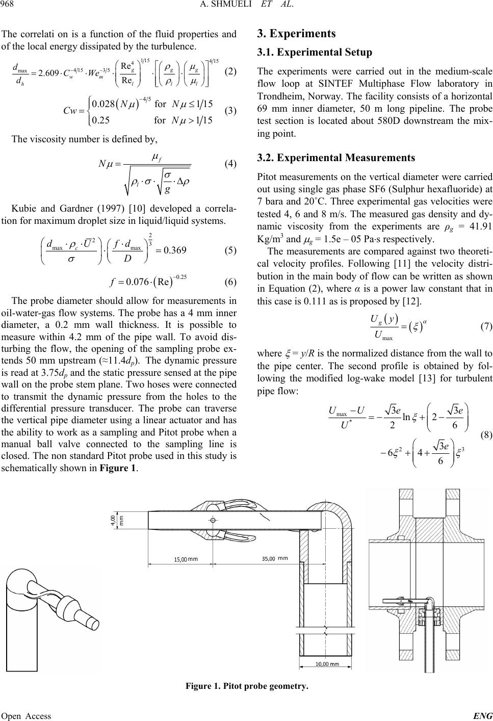

A. SHMUELI ET AL.

968

The correlati on is a function of the fluid properties and

of the local energy dissipated by the turbulence.

115 415

415 35

max Re

2.609 Re

ggg

dCWe











 















 ll

(2)



0.028for1 15

0.25for1 15

















(3)

The viscosity number is defined by,













 

(4)

Kubie and Gardner (1997) [10] developed a correla-

tion for maximum droplet size in liquid/liquid systems.

maxmax 0.369

dUfd







 









 (5)



0.25

0.076 Ref

 (6)

The probe diameter should allow for measurements in

oil-water-gas flow systems. The probe has a 4 mm inner

diameter, a 0.2 mm wall thickness. It is possible to

measure within 4.2 mm of the pipe wall. To avoid dis-

turbing the flow, the opening of the sampling probe ex-

tends 50 mm upstream (≈11.4dp). The dynamic pressure

is read at 3.75dp and the static pressure sensed at the pipe

wall on the probe stem plane. Two hoses were connected

to transmit the dynamic pressure from the holes to the

differential pressure transducer. The probe can traverse

the vertical pipe diameter using a linear actuator and has

the ability to work as a sampling and Pitot probe when a

manual ball valve connected to the sampling line is

closed. The non standard Pitot probe used in this study is

schematically shown in Figure 1.

3. Experiments

3.1. Experimental Setup

The experiments were carried out in the medium-scale

flow loop at SINTEF Multiphase Flow laboratory in

Trondheim, Norway. The facility consists of a horizontal

69 mm inner diameter, 50 m long pipeline. The probe

test section is located about 580D downstream the mix-

ing point.

3.2. Experimental Measurements

Pitot measurements on the vertical diameter were carried

out using single gas phase SF6 (Sulphur hexafluoride) at

7 bara and 20˚C. Three experimental gas velocities were

tested 4, 6 and 8 m/s. The measured gas density and dy-

namic viscosity from the experiments are ρg = 41.91

Kg/m3 and



g = 1.5e ‒ 05 Pas respectively.

The measurements are compared against two theoreti-

cal velocity profiles. Following [11] the velocity distri-

bution in the main body of flow can be written as shown

in Equation (2), where α is a power law constant that in

this case is 0.111 as is proposed by [12].

 

max





 (7)

where



= y/R is the normalized distance from the wall to

the pipe center. The second profile is obtained by fol-

lowing the modified log-wake model [13] for turbulent

pipe flow:

max

ln 2

UU ee





 













(8)

Figure 1. Pitot probe geometry.

Open Access ENG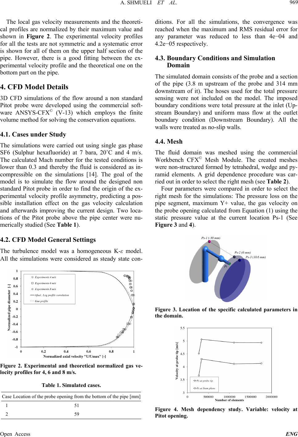

A. SHMUELI ET AL. 969

The local gas velocity measurements and the theoreti-

cal profiles are normalized by their maximum value and

shown in Figure 2. The experimental velocity profiles

for all the tests are not symmetric and a systematic error

is shown for all of them on the upper half section of the

pipe. However, there is a good fitting between the ex-

perimental velocity profile and the theoretical one on the

bottom part on the pipe.

4. CFD Model Details

3D CFD simulations of the flow around a non standard

Pitot probe were developed using the commercial soft-

ware ANSYS-CFX© (V-13) which employs the finite

volume method for solving the conservation equations.

4.1. Cases under Study

The simulations were carried out using single gas phase

SF6 (Sulphur hexafluoride) at 7 bara, 20˚C and 4 m/s.

The calculated Mach number for the tested conditions is

lower than 0.3 and thereby the fluid is considered as in-

compressible on the simulations [14]. The goal of the

model is to simulate the flow around the designed non

standard Pitot probe in order to find the origin of the ex-

perimental velocity profile asymmetry, predicting a pos-

sible installation effect on the gas velocity calculation

and afterwards improving the current design. Two loca-

tions of the Pitot probe above the pipe center were nu-

merically studied (See Table 1).

4.2. CFD Model General Settings

The turbulence model was a homogeneous K-ε model.

All the simulations were considered as steady state con-

Figure 2. Experimental and theoretical normalized gas ve-

locity profiles for 4, 6 and 8 m/s.

Table 1. Simulated cases.

Case Location of the probe opening from the bottom of the pipe [mm]

1 51

2 59

ditions. For all the simulations, the convergence was

reached when the maximum and RMS residual error for

any parameter was reduced to less than 4e−04 and

4.2e−05 respectively.

4.3. Boundary Conditions and Simulation

Domain

The simulated domain consists of the probe and a section

of the pipe (3.8 m upstream of the probe and 314 mm

downstream of it). The hoses used for the total pressure

sensing were not included on the model. The imposed

boundary conditions were total pressure at the inlet (Up-

stream Boundary) and uniform mass flow at the outlet

boundary condition (Downstream Boundary). All the

walls were treated as no-slip walls.

4.4. Mesh

The fluid domain was meshed using the commercial

Workbench CFX© Mesh Module. The created meshes

were non-structured formed by tetrahedral, wedge and py-

ramid elements. A grid dependence procedure was car-

ried out in order to select the right mesh (see Table 2).

Four parameters were compared in order to select the

right mesh for the simulations: The pressure loss on the

pipe segment, maximum Y+ value, the gas velocity on

the probe opening calculated from Equation (1) using the

static pressure value at the current location Ps-1 (See

Figure 3 and 4).

Figure 3. Location of the specific calculated parameters in

the domain.

Figure 4. Mesh dependency study. Variable: velocity at

Pitot opening.

Open Access ENG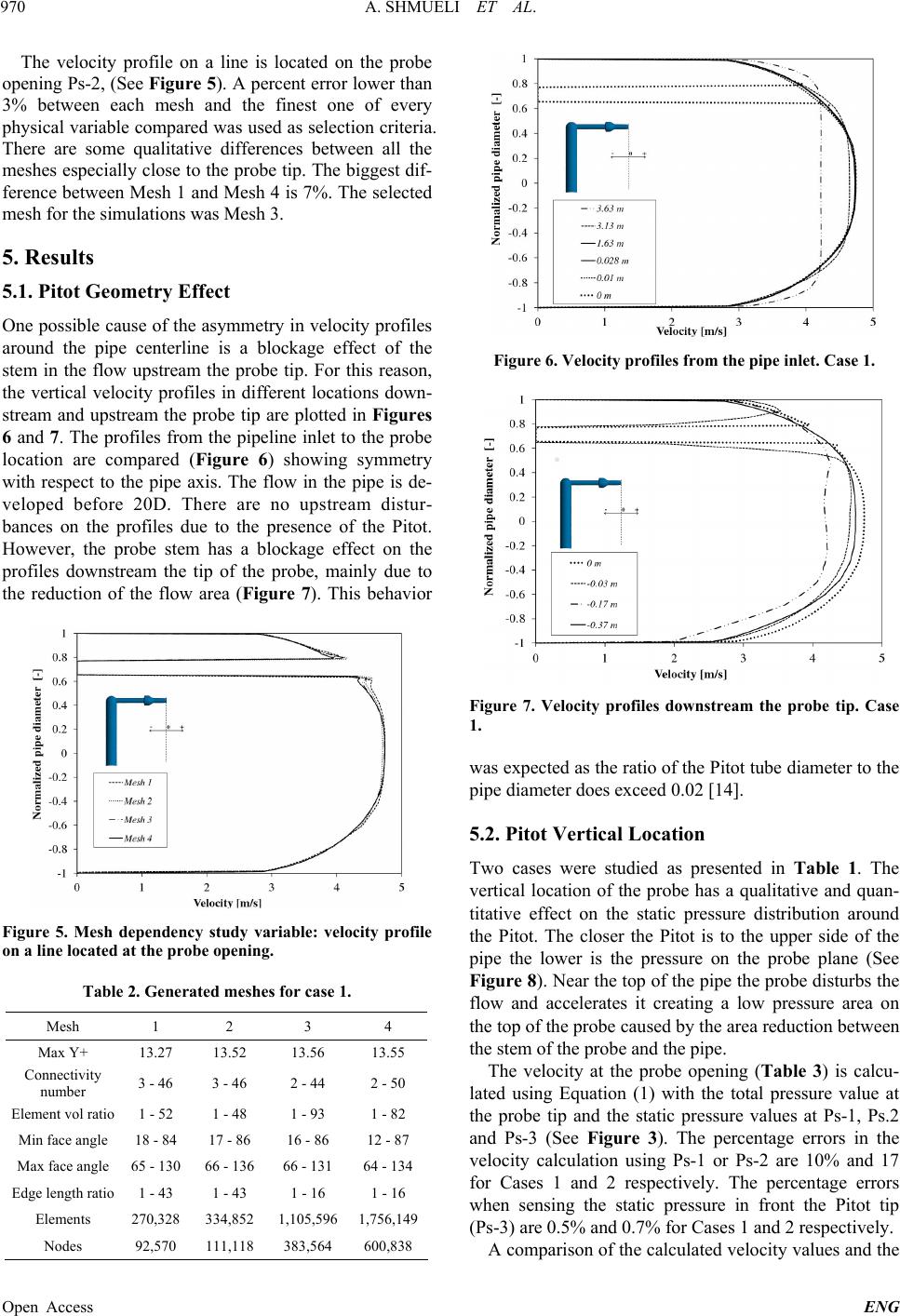

A. SHMUELI ET AL.

970

The velocity profile on a line is located on the probe

opening Ps-2, (See Figure 5). A percent error lower than

3% between each mesh and the finest one of every

physical variable compared was used as selection criteria.

There are some qualitative differences between all the

meshes especially close to the probe tip. The biggest dif-

ference between Mesh 1 and Mesh 4 is 7%. The selected

mesh for the simulations was Mesh 3.

5. Results

5.1. Pitot Geometry Effect

One possible cause of the asymmetry in velocity profiles

around the pipe centerline is a blockage effect of the

stem in the flow upstream the probe tip. For this reason,

the vertical velocity profiles in different locations down-

stream and upstream the probe tip are plotted in Figures

6 and 7. The profiles from the pipeline inlet to the probe

location are compared (Figure 6) showing symmetry

with respect to the pipe axis. The flow in the pipe is de-

veloped before 20D. There are no upstream distur-

bances on the profiles due to the presence of the Pitot.

However, the probe stem has a blockage effect on the

profiles downstream the tip of the probe, mainly due to

the reduction of the flow area (Figure 7). This behavior

Figure 5. Mesh dependency study variable: velocity profile

on a line located at the probe opening.

Table 2. Generated meshe s for case 1.

Mesh 1 2 3 4

Max Y+ 13.27 13.52 13.56 13.55

Connectivity

number 3 - 46 3 - 46 2 - 44 2 - 50

Element vol ratio 1 - 52 1 - 48 1 - 93 1 - 82

Min face angle 18 - 84 17 - 86 16 - 86 12 - 87

Max face angle 65 - 130 66 - 136 66 - 131 64 - 134

Edge length ratio 1 - 43 1 - 43 1 - 16 1 - 16

Elements 270,328 334,852 1,105,596 1,756,149

Nodes 92,570 111,118 383,564 600,838

Figure 6. Velocity profiles from the pipe inlet. Case 1.

Figure 7. Velocity profiles downstream the probe tip. Case

was expected as the ratio of the Pitot tube diameter to the

pipe diameter does exceed 0.02 [14].

5.2. Pitot Vertical Location

Two cases were studied as presented in Table 1. The

vertical location of the probe has a qualitative and quan-

titative effect on the static pressure distribution around

the Pitot. The closer the Pitot is to the upper side of the

pipe the lower is the pressure on the probe plane (See

Figure 8). Near the top of the pipe the probe disturbs the

flow and accelerates it creating a low pressure area on

the top of the probe caused by the area reduction between

the stem of the probe and the pipe.

The velocity at the probe opening (Table 3) is calcu-

lated using Equation (1) with the total pressure value at

the probe tip and the static pressure values at Ps-1, Ps.2

and Ps-3 (See Figure 3). The percentage errors in the

velocity calculation using Ps-1 or Ps-2 are 10% and 17

for Cases 1 and 2 respectively. The percentage errors

when sensing the static pressure in front the Pitot tip

(Ps-3) are 0.5% and 0.7% for Cases 1 and 2 respectively.

A comparison of the calculated velocity values and the

Open Access ENG

A. SHMUELI ET AL. 971

Figure 8. Static pressure contour case 2.

Table 3. Velocity at the probe opening calculated with total

pressure and static pressur e at point 1 and 2.

Case Location

Static Pressure

[Pa]

Total Pressure

[Pa]

Velocity at the

probe opening

[m/s]

Ps-1 699,344 - 4.92

Ps-2 699,428 - 4.49

Ps-3 699,434 4.46

Pt 699,851

Ps-1 699,003 - 4.89

Ps-2 699,151 - 4.10

Ps-3 699,156 4.08

Pt - 699,504 -

experimental one is made in Figure 9. Using the static

pressure at the probe tip plane to calculate the local ve-

locity shows a better fit with the theoretical profiles.

5.3. Pitot Probe Sampling under an Isokinetic

Condition

The main goal of this simulation was to obtain the pres-

sure loss inside the probe working under isokinetic con-

dition. It is important to establish the pressure loss be-

tween the probe tip and the dynamic pressure ports inside

it. For this simulation just Case 2 was analyzed.

The simulation and mesh selection was done following

the steps explained on section 4. The flow conditions and

fluid are the same as in the previous simulations. The

imposed boundary conditions were total pressure at the

inlet (Upstream Boundary), uniform mass flow at the

outlet of the probe (calculated from the isokinetic condi-

tion) and uniform mass flow at the outlet boundary con-

dition (Downstream Boundary). All the walls were treat-

ed as no-slip walls. The k-ε turbulence model was used

on the simulations.

The streamlines approaching the probe opening and

inside it are plotted in Figure 10. All the streamlines are

undisturbed as the probe is not present and the velocity

of the flow entering the probe is the same as in the main

body of the flow so the conditions for isokinetic sam-

pling are accomplished.

The total pressure is averaged on planes perpendicular

to the flow inside the probe (See Figure 11). The total

pressure holes are currently located on the position

marked by the dotted line. The pressure loss between the

probe opening and the total pressure holes is 33 Pa.

Figure 9. Comparison between experimental, theoretical

and CFD normalized gas velocity profile at 4 m/s.

Figure 10. Streamlines entering the probe.

Figure 11. Total pressure averaged on planes inside the

probe where location 1 is the probe opening.

Open Access ENG

A. SHMUELI ET AL.

972

6. Experiments on the Upgraded Installation

New experiments at 4 m/s were developed using an up-

graded setup in which the static pressure tap was located

on the same plane of the probe tip. The velocity profiles

are symmetric in accordance to the pipe axial direction.

The experiments are compared against the CFD profile

showing an agreement and improvement in comparison

with the previous setup (See Figure 12).

7. Conclusions and Remarks

A non-standard Pitot/sampling probe was experimentally

tested and simulated using Ansys CFX (V13) to validate

its accuracy and to determine any design or installation

problem. The current experimental setup caused asym-

metries on the measured gas velocity profiles.

The experiments were conducted for 3 velocities while

the numerical simulations were carried out for one veloc-

ity. The obtained experimental asymmetries show a sys-

tematic behavior so the numerical results are extrapolated

to other flow conditions.

The CFD simulations were concentrated on two probe

vertical locations where the velocity profiles present the

asymmetry. The effect of the probe location on the verti-

cal pipe diameter, static pressure port location on the

pipe wall, probe stem location and dynamic pressure

ports location was studied. The location of the static

pressure tap at either the probe tip plane or upstream of it

will give more real and accurate velocity values.

As a result from the simulations, the static pressure tap

at the top of the pipe was relocated in order to have a real

and accurate reading of the static pressure. The probe

itself generates disturbances of the flow downstream of it

but not upstream of it.

A simulation of the isokinetic sampling probe was car-

ried out to obtain the pressure drop inside the probe. It

Figure 12. Comparison of the experiments carried out the

upgraded facility at 4 m/s with previous experiments and

CFD profile.

was recommended for further probe designs to place the

dynamic pressure holes on the probe closer to the probe

tip in order to avoid the pressure losses and have a better

reading of the pressure.

Experiments with a new configuration with the static

pressure tap on the same plane as the probe tip were car-

ried out at 4 m/s showing an improvement on the meas-

urements with symmetric velocity profiles which agreed

with the theoretical predictions.

8. Acknowledgements

The financial and research support from Total E&P and

Sintef Petroleum Research are greatly appreciated.

REFERENCES

[1] L. A. Dykhno, “Maps of Mean Gas Velocity for Stratified

Flows with and without Atomization,” International

Journal of Multiphase Flow, Vol. 20, No. 4, 1994, pp

691-702.

http://dx.doi.org/10.1016/0301-9322(94)90039-6

[2] F. M. White, “Fluid Mechanics,” 4th Edition, McGraw-

Hill, New York, 1999.

[3] D. Tayebi, S. Nuland and P. Fuchs, “Droplet Transport in

Oil/Gas and Water/Gas at High Densities,” International

Journal of Multiphase Flow, Vol. 26. 2000, pp. 741-761.

http://dx.doi.org/10.1016/0301-9322(94)90039-6

[4] R. Skartlien, S. Nuland and J. Amundsen, “Simultaneous

Entrainment of Oil and Water Droplets in High Reynolds

Number Gas Turbulence in Horizontal Pipe Flow,” Inter-

national Journal of Multiphase Flow, Vol. 37 2011, pp.

1282-1293.

http://dx.doi.org/10.1016/j.ijmultiphaseflow.2011.07.006

[5] G. Falcone, F. Hewitt and C. Alimonti, “Multiphase Flow

Metering: Principles and Applications,” Elsevier, Amster-

dam, 2009.

[6] R. C. Baker, “Flow Measurement Handbook: Industrial

Designs, Operating Principles, Performance and Applica-

tions,” Cambridge University Press, New York, 2000.

http://dx.doi.org/10.1017/CBO9780511471100

[7] M. Wicks and A. E. Dukler, “Entrainment and Pressure

Drop in Concurrent Gas-Liquid Flow: Air-Water in Hori-

zontal Flow,” American Institute of Chemical Engineers,

Vol. 6, No. 10, 1960, pp. 463-468.

http://dx.doi.org/10.1002/aic.690060324

[8] L. Williams, “Effect of Pipe Diameter on Horizontal An-

nular Two-Phase Flow,” PhD Thesis, University of Illi-

nois at Urbana-Champaign, 1990.

[9] G. Kocamustafaogullari, S. R. Smits and J. Razi, “Maxi-

mum and Mean Droplet Sizes in Annular Two-Phase

Flow,” International Journal of Heat and Mass Transfer,

Vol. 37, No. 6, 1994, pp. 955-965.

http://dx.doi.org/10.1016/0017-9310(94)90220-8

[10] J. Kubie and G. C. Gardner, “Drop Sizes and Drop Dis-

persion in Straight Horizontal Tubes and Helical Coils,”

Chemical Engineering Science, Vol. 32, No. 2, 1977, pp.

195-202.

Open Access ENG

A. SHMUELI ET AL.

Open Access ENG

973

http://dx.doi.org/10.1016/0009-2509(77)80105-X

[11] N. Afzal, A. Seena and A. Bushra, “Power Law Velocity

Profile in Fully Developed Turbulent Pipe and Channel

Flows,” Journal of Hydraulic Engineering, Vol. 133, No.

9, 2007, pp. 1080-1086.

http://dx.doi.org/10.1061/(ASCE)0733-9429(2007)133:9(

1080)

[12] W. J. Duncan, A. B. Thorn and A. D. Young, “Mechanics

of Fluids,” ELBS Edward Arnold, 1967.

[13] J. Guo and P. Juliem, “Modified Log-Wake Law for Tur-

bulent Flow in Smooth Pipes,” Journal of Hydraulic Re-

search, Vol. 41, No. 4, 2003, pp. 493-501.

http://dx.doi.org/10.1080/00221680309499994

[14] ISO, “Measurement of Fluid Flow in Closed Conduits-

Velocity Area Method Using Pitot Static Tubes,” ISO

3966, 1977, pp. 146-183.

A. SHMUELI ET AL.

974

Appendix Nomenclature

ρ Density

P Pressure

d Diameter

D Pipe diameter

C Pitot calibration constant ≈ 1

U Velocity

R Pipe radius

Umax Velocity at the pipe center

dmax Maximum droplet size

dh Hydraulic diameter

dp Pitot diameter

Cw Coefficient in Kocamustafaogullari correlation

y Distance from the wall



Normalized distance from the wall to the pipe center



Dynamic viscosity



Power law constant

Re Reynolds number

f Friction factor

Wem Modified Weber number



Viscosity number



Surface tension

g Gravity

Subscripts

c Core

d Dynamic

s Static

t Total

g Gas

l Liquid

p Probe

Open Access ENG