A Simple Model for On-Sensor Phase-Detection Autofocusing Algorithm

doi:10.4236/jcc.2013.16003

Paper Menu >>

Journal Menu >>

Journal of Computer and Communications, 2013, 1, 11-17

Published Online November 2013 (http://www.scirp.org/journal/jcc)

http://dx.doi.org/10.4236/jcc.2013.16003

Open Access JCC

A Simple Model for On-Sensor Phase-Detection

Autofocusing Algorithm

Przemysław Śliwiński, Paweł Wachel

Institute of Computer Engineering, Control and Robotics, Wrocław University of Technology, Wrocław, Poland.

Email: [email protected], [email protected]

Received September 2013

ABSTRACT

A simple model of the phase-detection autofocus device based on the partially masked sensor pixels is described. The

cross-correla tion funct i on of the half-images registered by the masked pixels is proposed as a focus function. It is shown

that—in such setting—focusing is equivalent to searching of the cross-correlation function maximum. Application of

stochastic approximation algorithms to unimodal and non-unimodal focus functions is shortly discussed.

Keywords: Phase Detection Autofocus; On-Sensor Circuit; Formal Model; Cros s-Correlation; Stochastic

Approximation

1. Introduction

In imaging, focusing can be defined as seeking for the

image being the best approximation of the captured scene.

The proposed autofocusing algorithm is of a stochastic

optimization type. Within the stochastic framework we

model the scene as a random process (continuous, s ta-

tionary and fourth-order) of an unknown distribution1.

Assuming that the dimensions of the lens and sensors are

far larger than the length of the light-wave we can use the

first order (geometric/linear) approximation of the optics

laws [1,2]. In particular, we can model the lens as a li-

near low-pass filter with a symmetric (box) impulse re-

sponse centered at the origin [3]. The width of the box is

therefore proportional to the distance between the sensor

and the image plane. One can note that the scene is “in

focus” when the sensor is in the image plane, that is, in

the plane where all rays from a single point at the scene

converge into a single point (and the corresponding im-

pulse response of the lens is the Dirac delta function).

A popular approach to this problem in digital imaging

is to use the sequentially collected images with their va-

riance serving as a focus function. Such an approach is

referred to as the contrast-detection auto-focusing (we

will use the common CD AF acronym for shortness)

which also includes algorithms based on an image histo-

gram or its gradient analysis. It does not require any ad-

ditional equipment and hence can be implemented in

virtually all digital cameras. Its well-known issue, how-

ever, is that a single image does not provide information

about either:

• the distance between the sensor and the image plane,

• the direction toward the sensor should be shifted in

order to attain a focused image,

and subsequently CD algorithms seek the focus itera-

tively, in the back-and-forth manner (shifting the lens

accordingly), and require capturing an image in each

position determined by the algorithm. The CD AF algo-

rithms are usually derivatives of the stochastic approxi-

mation routines (like e.g. the golden-section search (if a

noise is negligible) or the Kiefer-Wolfowitz algorithm (if

the noise impact cannot be ignored) [4,5]). In conse-

quence, they are rather slow and not directly applicable

in e.g. object tracking or video applications.

In order to overcome these deficiencies one can use

algorithms based on the phase-detection auto-focusing

(PD AF) principle, in which a single image is split into

two, lef t- and right-hand side halves. Typically, image

splitting is achieved with the help of a separate optical

path consisting of semi-transparent/pellicle mirrors and

dedicated line sensors and such an implementation is

often met in digital SLRs; see e.g. [3]). The half-images

—if the scene is out-of-focus—are shifted with respect to

each other. Such a shift is traditionally referred to as a

“phase shift” and maintains information about both:

• the distance between the sensor and the image plane,

and

• the direction towards the sensor should be moved.

1For simplicity, we consider a 1D case rather than the full 2D one.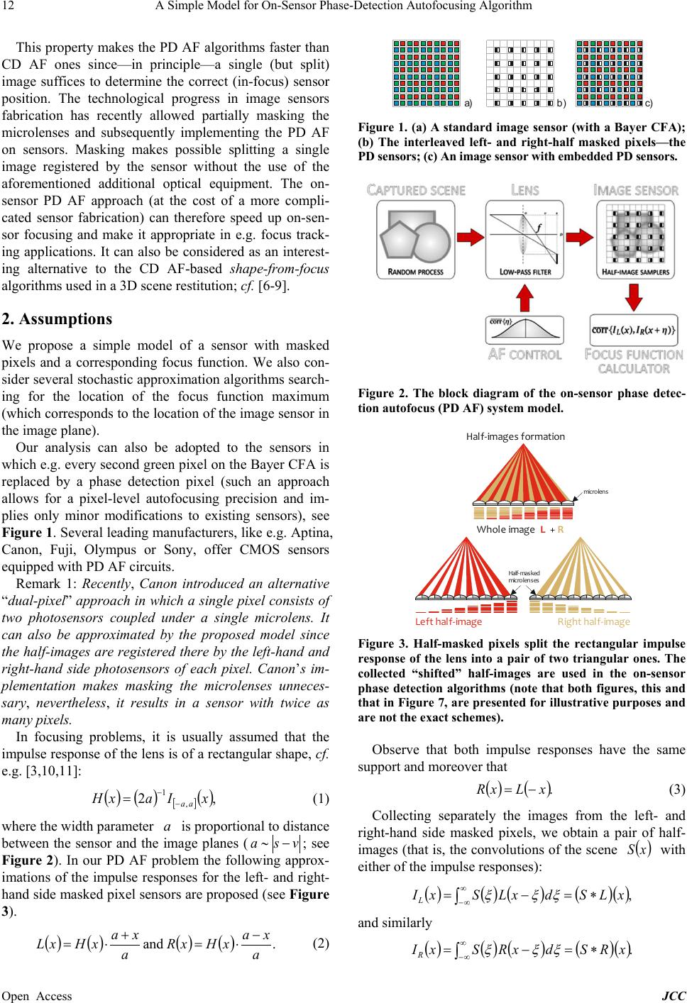

A Simple Model for On-Sensor Phase-Detection Autofocusing Algorithm

Open Access JCC

This property makes the PD AF algorithms faster than

CD AF ones since—in principle—a single (but split)

image suffices to determine the correct (in-focus) sensor

position. The technological progress in image sensors

fabrication has recently allowed partially masking the

microlenses and subsequently implementing the PD AF

on sensors. Masking makes possible splitting a single

image registered by the sensor without the use of the

aforementioned additional optical equipment. The on-

sensor PD AF approach (at the cost of a more compli-

cated sensor fabrication) can therefore speed up on-sen-

sor focusing and make it appropriate in e.g. focus track-

ing applications. It can also be considered as an interest-

ing alternative to the CD AF-based shape-from-focus

algorithms used in a 3D scene restitution ; cf. [6-9].

2. Assumptions

We propose a simple model of a sensor with masked

pixels and a corresponding focus function. We also con-

sider several stochastic ap proximation algorithms search -

ing for the location of the focus function maximum

(which corresponds to the location of the image sensor in

the image plane).

Our analysis can also be adopted to the sensors in

which e.g. every second green pixel on the Bayer CFA is

replaced by a phase detection pixel (such an approach

allows for a pixel-level autofocusing precision and im-

plies only minor modifications to existing sensors), see

Figure 1. Several leading manufacturers, like e.g. Aptina,

Canon, Fuji, Olympus or Sony, offer CMOS sensors

equippe d with PD AF cir cuits.

Remark 1: Recently, Canon introduced an alternative

“dual-pixel” approach in which a single pixel consists of

two photosensors coupled under a single microlens. It

can also be approximated by the proposed model since

the half-images are registered there by the left-hand and

right-hand side photosensors of each pixel. Canon’s im-

plementation makes masking the microlenses unneces-

sary, nevertheless, it results in a sensor with twice as

many pixels.

In focusing problems, it is usually assumed that the

impulse response of the lens is of a rectangular shape, cf.

e.g. [3,10,11]:

( )()

[ ]

( )

xIaxH

aa−

−

(1)

where the width parameter

is proportional to distance

between the sensor and the image planes (

vsa −∼

; see

Figure 2). In our PD AF problem the following approx-

imations of the impulse responses for the left- and right-

hand side masked pixel sensors are proposed (see Figure

3).

( )( )( )( )

. and a

xHxR

xHxL −

⋅=

(2)

Figure 1. (a) A standard image sensor (with a Bayer CFA);

(b) The interleaved left- and right-half masked pixels—the

PD sensors; (c) An image sensor with embedded PD sensors.

Figure 2. The block diagram of the on-sensor phase detec-

tion autofocus (PD AF) system model.

Figure 3. Half-masked pixels split the rectangular impulse

response of the lens into a pair of two triangular ones. The

collected “shifted” half-images are used in the on-sensor

phase detection algorithms (note that both figures, this and

that in Figure 7, are presented for illustrative purposes and

are not the exact schemes).

Observe that both impulse responses have the same

support and moreover that

( )()

.xLxR −=

(3)

Collecting separately the images from the left- and

right-hand side masked pixels, we obtain a pair of half-

images (that is, the convolutions of the scene

( )

with

either of the impulse responses):

( )()()()( )

,xLSdxLSxI

∗=−= ∫

∞

∞−

ξξξ

and similarly

( )()()()( )

.xRSdxRSxI

∗=−= ∫

∞

∞−

ξξξ

a) b) c)

Left half-image

Half-images formation

Right half-image

Whole image + L R

mic ro len s

Half- mas ked

microlenses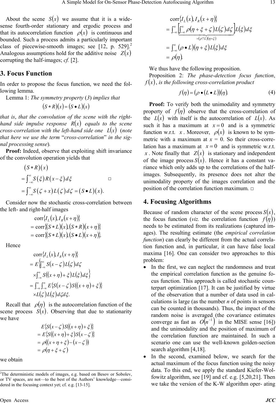

A Simple Model for On-Sensor Phase-Detection Autofocusing Algorithm

Open Access JCC

About the scene

( )

we assume that it is a wide-

sense fourth-order stationary and ergodic process and

that its autocorrelation function

( )

is continuous and

bounded. Such a process admits a particularly important

class of piecewise-smooth images; see [12, p. 529].2

Analogous assumptions hold for the additive noise

( )

corrupting the half-images; cf. [2].

3. Focus Function

In order to propose the focus function, we need the fol-

lowing lemma.

Lemma 1: The symmetry property (3) implies that

()( )()( )

xLSxRS •=∗

that is, that the convolution of the scene with the right-

hand side impulse response

( )

equals to the scene

cross-correlation with the left-hand side one

( )

(note

that here we use the term “cross-correlation” in the sig-

nal proces s ing sense).

Proof: Inde ed, observe that exploiting shift invariance

of the convolution operation yields that

()( )

( )()

() ()()( )

SRx

S Rxd

SxLdSLx

ξ ξξ

ζ ζζ

∞

−∞

∞

−∞

∗

= −

=+=•

∫

□

Consider now the stochastic cross-correlation between

the left- and right-half images

( )(){}

()() ()(){}

( )()( )(){}

.,corr

,corr

+•∗=

+∗∗=

xLSxLS

xRSxLS

xIxI

Hence

( )(){}

()()

{

()()( )

}

()()(){}

()()

,corr

ξζξζ

ξηζ

ξξξη

ζζζ

ddLL

xSxSE

dLxS

dLxSE

xIxI

++−=

++×

−=

∫∫

∫

∞

∞−

∞

∞−

∞

∞−

∞

∞−

Recall that

( )

ηρ

is the autocorrelation function of the

scene process

( )

. Observing that due to stationarity

we have

() ()(){}

()() (){}

() ()()

( )

ζξηρ

ζξη

ξηζ

++=

−−++=

−++=

++−

xSxSE

we obtain

( )(){}

() ( )

[ ]

()( )

( )

()()( )

( )

,corr

ηρ

ξξξηρ

ξξζζζξηρ

ξηρ

+•=

++=

∫

∫∫

∞

∞−

∞

∞−

∞

∞−

dLL

dLdL

xIxI

  

We thus have the following proposition.

Proposition 2: The phase-detection focus function,

( )

, is the following cross-correlatio n pr oduct

( )()()( )

ηρη

LLf ••=

(4)

Proof: To verify both the unimodality and symmetry

property of

( )

observe that the cross-correlation of

the

( )

with itself is the autocorrelation of

( )

. As

such it has a maximum at

0=x

and is a symmetric

function w.r.t.

. Moreover,

( )

is known to be sym-

metric with a maximum at x = 0. So their cross-corre-

lation has a maximum at

0=x

and is symmetric w.r.t.

. Note finally that

( )

is stationary and independent

of the image process

( )

. Hence it has a constant va-

riance which only adds up to the correlations of the half-

images. Subsequently, its presence does not alter the

unimodality property of the images correlation and the

position of the correlation function maximum. □

4. Focusing Algorithms

Because of random character of the scene process

( )

the focus function (viz. the correlation function

( )

)

needs to be estimated from its realizations (captured im-

ages). The resulting estimate (the empirical correlation

function) can clearly be different from the actual correla-

tion function and, in particular, it can have false local

maxima [16]. One can consider two approaches to this

problem:

• In the first, we can neglect the randomness and treat

the empirical correlation function as the genuine fo-

cus function. This approach is called stochastic coun-

terpart optimization [17]. It can be justified by virtue

of the observation that a number of data used in cal-

culations is large (as the number n of points in se nsors

can be counted in thousands). Thus, th e impact of the

random noise is averaged (the covariance estimates

converge as fast as

( )

1−

in the MISE sense [16])

and the unimodality and the position of maximum of

the correlation function are maintained. In such a

scenario one can use the well-known golden-section

search algorithm [4,18].

• In the second, examined below, we search for the

actual maximum of the focus function using the noisy

data. To this end, we apply the standard Kiefer-Wol-

fowitz algorithm, see [19] and cf. e.g. [5,20,21]. Then

we take the version of the K-W algorithm oper- ating

2The

deterministic models of images, e.g. based on Besov or Sobolev,

or TV spaces, are not—to the best of the Authors’ knowledge—consi-

dered in the focusing context yet; cf. e.g. [13-15].

A Simple Model for On-Sensor Phase-Detection Autofocusing Algorithm

Open Access JCC

on the smoothed functional as in [22-23] and cf.

[24,25], in order to apply the algorithm to the case

when the correlation function is not unimodal.

4.1. Unimodal Case

Since the focus function

( )

in (4) is unimodal by

assumption, to apply Kiefer-Wolfowitz stochastic appro-

ximation algorithm, we merely need to assure that

( )

is also sufficiently smooth. Recalling that

( )

is itself

the correlation of the continuous and bounded function

()( )

xLL•

with the continuous and bounded autocorrela-

tion function

( )

, we infer that

( )

has at least one

bounded derivative, that is, it satisfies the Kiefer-Wol-

fowitz convergence conditions.

4.2. Multimodal Case

Let the autocorrelation function of the scene process

( )

be multimodal.3 Then, the focus function

( )

(4) is no longer unimodal and the standard stochastic

approximation algorithms fail in general and find local

maxima. We show that by convolving

( )

with a rec-

tangular kernel (box) function, we obtain a (smoothed)

version of

( )

which gains unimodality property and

maintains the position of the maximum of

( )

; cf. [22].

The following lemma gives sufficient conditions for the

focus and kernel funct i ons,

( )

and

( )

Lemma 3: Let

( )

[ ]

( )

xIrxh

rr,

−

and let

( )

a multimodal focus function with the global maximum at

0, with a support included in [−r, r]. Then, the convolu-

tion

()( )

xfh∗

is unimodal with the maximum at 0.4

By assumption, f(x) has a global maximum at 0. Let

F(x) denote its primitive function. The convolution of f(x)

with a rectangular kernel

( )

of support [−r, r] equals

()( )( )() ()

rxFrxF

xfh

−−+

==∗ ∫

−

ξξ

If, for all

>− rx

and

,yx <

the following differ-

ences are negative

()()() ()

22 <

−−+

−

−−+

rxFrxF

ryFryF

that is if

() ()() ()

,rxFrxFryFryF−−+<−−+

(5)

then the convolution is unimodal (since it also is symme-

tric). Since the support of

( )

is at most [−r, r], then

for any

0, >yx

, we have that

( )( )

,ryFryF +=+

and

the condition in (5) reduces to

() ()

rxFryF

−>−

which holds for any

0, >yx

, as

( )

is non-negative

(and

( )

non-decreasing) and

yx <

5. Numerical Simulations

The hardware equipped with the on-sensor PD pixels has

not been available to Authors at the time of the paper

preparation. Therefore, we performed a simple numerical

experiment illustrating the approach and based on a sty-

lized model in the environment provided by the Mathe-

matica and C++ packages. A sample scene

( )

is pre-

sented in Figure 4 together with the half-images,

( )

and

( )

. Figure 5 shows the shape of the resulting fo-

cus function

( )

. In Figure 6 the results of application

of the Kiefer-Wolfowitz algorithms are shown for the

sequences

( )

1−

=nna

and

( )

3/1−

=nnc

(as in the orig-

inal algorithm in [19]). The white noise of uniform dis-

tribution in the interval

[ ]

1.0,1.0− was added to the

focus func t ion.

6. Final Remarks

In the classic paper by Krotkov [26], several criteria of

Figure 4. The sam ple scene (black li ne), and its left (brown)

and right (r ed) half-images.

Figure 5. The focus function of the scene from Figure 4.

3But still symmetric—due to stationarity of S(x).

4If f(x) is not symmetric, the convolution with such h(x) remains un-

imodal with the maximum at o rigin, bu t this po int may no lo nger be th e

actual maximum of the focus function.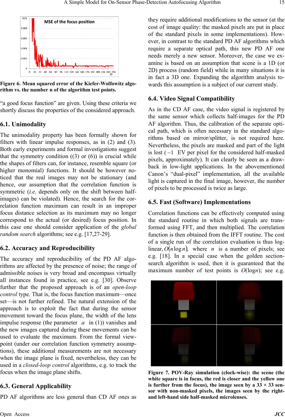

A Simple Model for On-Sensor Phase-Detection Autofocusing Algorithm

Open Access JCC

Figure 6. Mean squared error of the Kiefer-Wolfowitz algo-

rithm vs. the number n of the algorithm test points.

“a good focus function” are given. Usin g these criteria we

shortly discuss the properties of the considered approach.

6.1. Unimodality

The unimodality property has been formally shown for

filters with linear impulse responses, as in (2) and (3).

Both early experiments and formal investigations sugges t

that the symmetry condition ((3) or (6)) is crucial while

the shapes of filters can, for instan ce , resemble square (or

higher monomial) functions. It should be however no-

ticed that the real images may not be stationary (and

hence, our assumption that the correlation function is

symmetric (i.e. depends only on the shift between half-

images) can be violated). Hence, the search for the cor-

relation function maximum can result in an improper

focus distance selection as its maximum may no longer

correspond to the actual (or desired) focus position. In

this case one should consider application of the global

random search algorithms; see e.g. [17,27-29].

6.2. Accuracy and Reproducibility

The accuracy and reproducibility of the PD AF algo-

rithms are affected by the presence of noise; the r ange of

admissible noises is very broad and encompass virtually

all instances found in practice, see e.g. [30]. Observe

further that the proposed approach is of an open-loop

control type. That is, the focus function maximum—once

set—is not further refined. The natural extension of the

approach is to exploit the fact that during the sensor

movement toward the focus plane, the width of the lens

impulse respons e (the para meter

in (1)) vanishes and

the new images captured during these movements can be

used to evaluate the maximum. From the formal view-

point (under our correlation function symmetry assump-

tions), these additional measurements are not necessary

when the image plane is fixed, nevertheless, they can be

used in a closed-loop control algorithms, e. g. to track the

focus when the image plane shifts.

6.3. General Applicability

PD AF algorithms are less general than CD AF ones as

they require additional modif ications to the sensor (at the

cost of image quality: the masked pixels are put in place

of the standard pixels in some implementations). How-

ever, in contrast to the standard PD AF algorithms which

require a separate optical path, this new PD AF one

needs merely a new sensor. Moreover, the case we ex-

amine is based on an assumption that scene is a 1D (or

2D) process (random field) while in many situations it is

in fact a 3D one. Expanding the algorithm analysis to-

wards this assumption is a subject of our curre nt study.

6.4. Video Signal Compatibility

As in the CD AF case, the video signal is registered by

the same sensor which collects half-images for the PD

AF algorithm. Thus, the calibration of the separate opti-

cal path, which is often necessary in the standard algo-

rithms based on mirror/splitter, is not required here.

Nevertheless, the pixels are masked and part of the light

is lost (

1−

EV per pixel for the considered half-masked

pixels, approximately). It can clearly be seen as a draw-

back in low-light applications. In the abovementioned

Canon’s “dual-pixel” implementation, all the available

light is captured in the final image, however, the number

of pixels to be processed is twice as large.

6.5. Fast (Software) Implementations

Correlation functions can be effectively computed using

the standard routine in which both signals are trans-

formed using FFT, and then multiplied. The correlation

function is then obtained from the IFFT routine. The cost

of a single run of the correlation evaluation is thus log-

linear,

( )

,lo gnnO where

is a number of pixels; see

e.g. [18]. In a special case when the golden section-

search algorithm is used, then it is guaranteed that the

maximum number of test points is O(logn); see e.g.

Figure 7. POV-Ray simulation (clock-wise): the scene (the

white square is in focus, the red is closer and the yell ow one

is further from the focus), the image seen by a 33 × 33 sen-

sor with non-masked pixels, the images seen by the right-

and left-hand si de half-masked microlenses.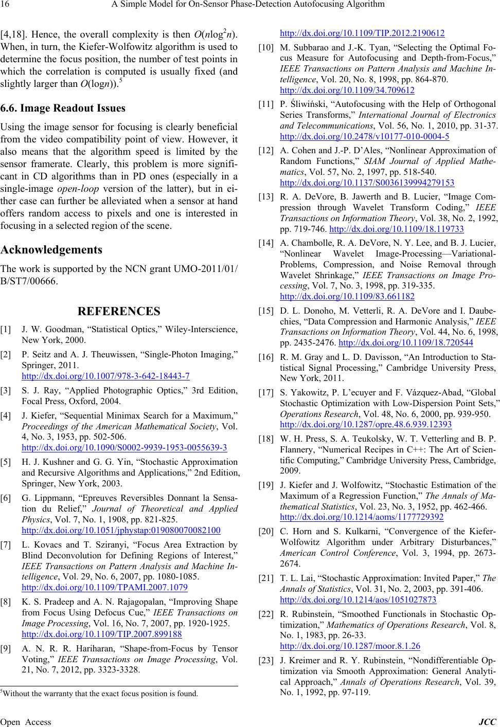

A Simple Model for On-Sensor Phase-Detection Autofocusing Algorithm

Open Access JCC

[4,18]. Hence, the overall complexity is then O(nlog2n).

When, in turn, the Kief er-Wolfowitz algorithm is used to

determine the focus position , the number of test points in

which the correlation is computed is usually fixed (and

slightly larger than O(logn)).5

6.6. Image Readout Issues

Using the image sensor for focusing is clearly beneficial

from the video compatibility point of view. However, it

also means that the algorithm speed is limited by the

sensor framerate. Clearly, this problem is more signifi-

cant in CD algorithms than in PD ones (especially in a

single-ima g e open-loop version of the latter), but in ei-

ther case can further be alleviated when a sensor at hand

offers random access to pixels and one is interested in

focusing in a selected region of the scene.

Acknowledgements

The work is supported by the NCN gran t UMO-2011/01/

B/ST7/00666 .

REFERENCES

[1] J. W. Goodman, “Statistical Optics,” Wiley-Interscience,

New York, 2000.

[2] P. Seitz and A. J. Theuwissen, “Single-Photon Imaging,”

Springer, 2011.

http://dx.doi.org/10.1007/978-3-642-18443-7

[3] S. J. Ray, “Applied Photographic Optics,” 3rd Edition,

Focal Pre ss , Oxford, 2004.

[4] J. Kiefer, “Sequential Minimax Search for a Maximum,”

Proceedings of the American Mathematical Society, Vol.

4, No. 3, 1953, pp. 502-506.

http://dx.doi.org/10.1090/S0002-9939-1953-0055639-3

[5] H. J. Kushner and G. G. Yin, “Stochastic Approximation

and Recursive Algorithms and Applications,” 2nd Edition,

Springer, New York, 2003.

[6] G. Lippmann, “Epreuves Reversibles Donnant la Sensa-

tion du Relief,” Journal of Theoretical and Applied

Physics, Vol. 7, No. 1, 1908, pp. 821-825.

http://dx.doi.org/10.1051/jphystap:019080070082100

[7] L. Kovacs and T. Sziranyi, “Focus Area Extraction by

Blind Deconvolution for Defining Regions of Interest,”

IEEE Transactions on Pattern Analysis and Machine In-

telligence, Vol. 29, No. 6, 2007, pp. 1080-1085.

http://dx.doi.org/10.1109/TPAMI.2007.1079

[8] K. S. Pradeep and A. N. Rajagopalan, “Improving Shape

from Focus Using Defocus Cue,” IEEE Transactions on

Image Processing, Vol. 16, No. 7, 2007, pp. 1920-1925.

http://dx.doi.org/10.1109/TIP.2007.899188

[9] A. N. R. R. Hariharan, “Shape-from-Focus by Tensor

Voting,” IEEE Transactions on Image Processing, Vol.

21, No. 7, 2012, pp. 3323-3328.

http://dx.doi.org/10.1109/TIP.2012.2190612

[10] M. Subbarao and J.-K. Tyan, “Selecting the Optimal Fo-

cus Measure for Autofocusing and Depth-from-Focus,”

IEEE Transactions on Pattern Analysis and Machine In-

telligence, Vol. 20, No. 8, 1998, pp. 864-870.

http://dx.doi.org/10.1109/34.709612

[11] P. Śliwiński, “Autofocusing with the Help of Orthogonal

Series Transforms,” International Journal of Electronics

and Telecommunications, Vol. 56, No. 1, 2010, pp. 31-37.

http://dx.doi.org/10.2478/v10177-010-0004-5

[12] A. Cohen and J.-P. D’Ales, “Nonlinear Approximation of

Random Functions,” SIAM Journal of Applied Mathe-

matics, Vol. 57, No. 2, 1997, pp. 518-540.

http://dx.doi.org/10.1137/S0036139994279153

[13] R. A. DeVore, B. Jawerth and B. Lucier, “Image Com-

pression through Wavelet Transform Coding,” IEEE

Transactions on Information Theory, Vol. 38, No. 2, 1992,

pp. 719-746. http://dx.doi.org/10.1109/18.119733

[14] A. Chambolle, R. A. DeVore, N. Y. Lee, and B. J. Lucier,

“Nonlinear Wavelet Image-Processing—Variational-

Problems, Compression, and Noise Removal through

Wavelet Shrinkage,” IEEE Transactions on Image Pro-

cessing, Vol. 7, No. 3, 1998, pp. 319-335.

http://dx.doi.org/10.1109/83.661182

[15] D. L. Donoho, M. Vetterli, R. A. DeVore and I. Daube-

chies, “Data Compression and Harmonic Analy sis,” IEEE

Transactions on Information Theory, Vol. 44, No. 6, 1998,

pp. 2435-2476. http://dx.doi.org/10.1109/18.720544

[16] R. M. Gray and L. D. Davisson, “An Introduction to Sta-

tistical Signal Processing,” Cambridge University Press,

New York, 2011.

[17] S. Yakowitz, P. L’ecuyer and F. Vázquez-Abad, “Global

Stochastic Optimization with Low-Dispersion Point Sets,”

Operations Re search, Vol. 48, No. 6, 2000, pp. 939 -950.

http://dx.doi.org/10.1287/opre.48.6.939.12393

[18] W. H. Press, S. A. Teukolsky, W. T. Vetterling and B. P.

Flannery, “Numerical Recipes in C++: The Art of Scien-

tific Computing,” Cambridge University Press, Cambridge,

2009.

[19] J. Kiefer and J. Wolfowitz, “Stochastic Estimation of the

Maximum of a Regression Function,” The Annals of Ma-

thematical Statistics, Vol. 23, No. 3, 1952, pp. 462-466.

http://dx.doi.org/10.1214/aoms/1177729392

[20] C. Horn and S. Kulkarni, “Convergence of the Kiefer-

Wolfowitz Algorithm under Arbitrary Disturbances,”

American Control Conference, Vol. 3, 1994, pp. 2673-

2674.

[21] T. L. Lai, “St oc hast ic Approximation: Invited Paper,” The

Annals of Statistics, Vol. 31, No. 2, 2003, pp. 391-406.

http://dx.doi.org/10.1214/aos/1051027873

[22] R. Rubinstein, “Smoothed Functionals in Stochastic Op-

timization,” Mathematics of Operations Research, Vol. 8,

No. 1, 1983, pp. 26-33.

http://dx.doi.org/10.1287/moor.8.1.26

[23] J. Kreimer and R. Y. Rubinstein, “Nondifferentiable Op-

timization via Smooth Approximation: General Analyti-

cal Approach,” Annals of Operations Research, Vol. 39,

No. 1, 1992, pp. 97-119.

5Without the warranty that the exact focus position is found.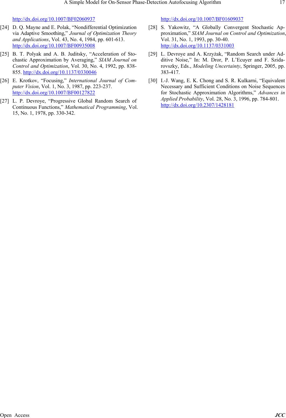

A Simple Model for On-Sensor Phase-Detection Autofocusing Algorithm

Open Access JCC

http://dx.doi.org/10.1007/BF02060937

[24] D. Q. Mayne and E. Polak, “Nondifferential Optimization

via Adaptive Smoothing,” Journal of Optimization Theory

and Applications, Vol. 43, No. 4, 1984, pp. 601-613.

http://dx.doi.org/10.1007/BF00935008

[25] B. T. Polyak and A. B. Juditsky, “Acceleration of Sto-

chastic Approximation by Averaging,” SIAM Journal on

Control and Optimization, Vol. 30, No. 4, 1992, pp. 838-

855. http://dx.doi.org/10.1137/0330046

[26] E. Krotkov, “Focusing,” International Journal of Com-

puter Vision, Vol. 1, No. 3, 1987, pp. 223-237.

http://dx.doi.org/10.1007/BF00127822

[27] L. P. Devroye, “Progressive Global Random Search of

Continuous Functions,” Mathematical Programming, Vol.

15, No. 1, 1978, pp. 330-342.

http://dx.doi.org/10.1007/BF01609037

[28] S. Yakowitz, “A Globally Convergent Stochastic Ap-

proximation,” SIAM Journal on Control and Optimization,

Vol. 31, No. 1, 1993, pp. 30-40.

http://dx.doi.org/10.1137/0331003

[29] L. Devroye and A. Krzyżak, “Random Search under Ad-

ditive Noise,” In: M. Dror, P. L’Ecuyer and F. Szida-

rovszky, Eds., Modeling Uncertainty, Springer, 2005, pp.

383-417.

[30] I.-J. Wang, E. K. Chong and S. R. Kulkarni, “Equivalent

Necessary and Sufficient Conditions on Noise Sequences

for Stochastic Approximation Algorithms,” Advances in

Applied Probability, Vol. 28, No. 3, 1996, pp. 784-801.

http://dx.doi.org/10.2307/1428181