An Empirical Study of Good-Turing Smoothing for Language Models on Different Size Corpora of Chinese

doi:10.4236/jcc.2013.15003

Paper Menu >>

Journal Menu >>

Journal of Computer and Communications, 2013, 1, 14-19

http://dx.doi.org/10.4236/jcc.2013.15003 Published Online October 2013 (http://www.scirp.org/journal/jcc)

An Empirical Study of Good-Turing Smoothing for

Language Models on Different Size Corpora of Chinese

Feng-Long Huang1, Ming-Shing Yu2, Chien-Yo Hwang2

1Department of Computer Science and Information Engineering, National United University, MaioLi, Chinese Taipei; 2Depa rtment

of Computer Science, National Chung-Hsing University, Taichung, Chinese Tai pei.

Email: [email protected], [email protected]

Received September 2013

ABSTRACT

Data sparseness has been an inherited issue of statistical language models and smoothing method is usually used to re-

solve the zero count problems. In this paper, we studied empirically and analyzed the well-known smoothing methods

of Good-Turing and advanced Good-Turing for language models on large sizes Chinese corpus. In the paper, ten mod-

els are generated sequentially on various size of corpus, from 30 M to 300 M Chinese words of CGW corpus. In our

experiments, the smoothing methods; Good-Turing and Advanced Good-Turing smoothing are evaluated on inside

testing and outside testing. Based on experiments results, we analyzed further the trends of perplexity of smoothing

methods, which are useful for employing the effective smoothing methods to alleviate the issue of data sparseness on

various sizes of language models. Finally, some helpful observations are described in detail.

Keywords: Good-Turing Methods; Smoothing; L a n guage M ode l s; Perplexity

1. Introduction

Speech processing (SP) studies the domain of speech

signals and the processing methods of these digital sig-

nals. It is always combined into natural language pro-

cessing (NLP). The technology development is wide-

spread day after day; the information system with speech

service already became important tendency. Speech Pro-

cessing may divide into two broad domains: Speech Re-

cognition and speech synthesis. The former is to recog-

nize the speech signal with respect to the text output and

the latter is to synthesize the speech with frequent pros-

ody for the text or articles inputs.

In many domains of natural language processing

(NLP); su ch as speech recognition [1], and machine tran-

slation [2]; the statistical language models (LMs) [3] play

an important role in na t ural la ng uage processing .

1.1. Language Models

The statistical language models have been widely used in

NLP. Supposed that W = w1, w2, w3, … wn, where wi and

n denote the the ith Chinese character and its number in a

sentence (

0in≤≤

). P(W) = P(w1, w2, ..., wn), the prob-

ability can be calculated by using chain rules:.

2( 1)

11 21 311

(() (|) (|)...()

)

PwPw Pww PwwPww

Pww

−

∏

(1)

where

−

denotes string w1, w2, w3, … wk−1.

In general, unigram, bigram and trigram (3 <= N) are

generated. N-gram model calculates P(•) of Nth events by

the preceding N − 1 events, rather than the string w1, w2,

w3 … wN-1.

1.2. N-Gram Models

Basically, N-gram is so-called N − 1)th—order Markov

model, which calculate co nditional probability of succes-

sive events: calculate the probability of Nth event while

preceding (N − 1) event oc curs.

Basically, N-gram Language Model is simply ex-

pressed as follows:

(|() )

k kN

wPw wP

−

−+

≈∏

(2)

()

(| )()

ii i

Cw w

Pw wCw w

−

∑

(3)

where C(w) denotes the counts of event w occurring in

dataset.

In formula (3), the obtained probability P(•) is so

called Maximum Likelihood Estimation (MLE). While

predicting the pronunciation category, we can predict

based on the probability on each category t (

1tT≤≤

), T

denotes the number of categories for the polyphonic

character. The category with maximum probability Pmax(•)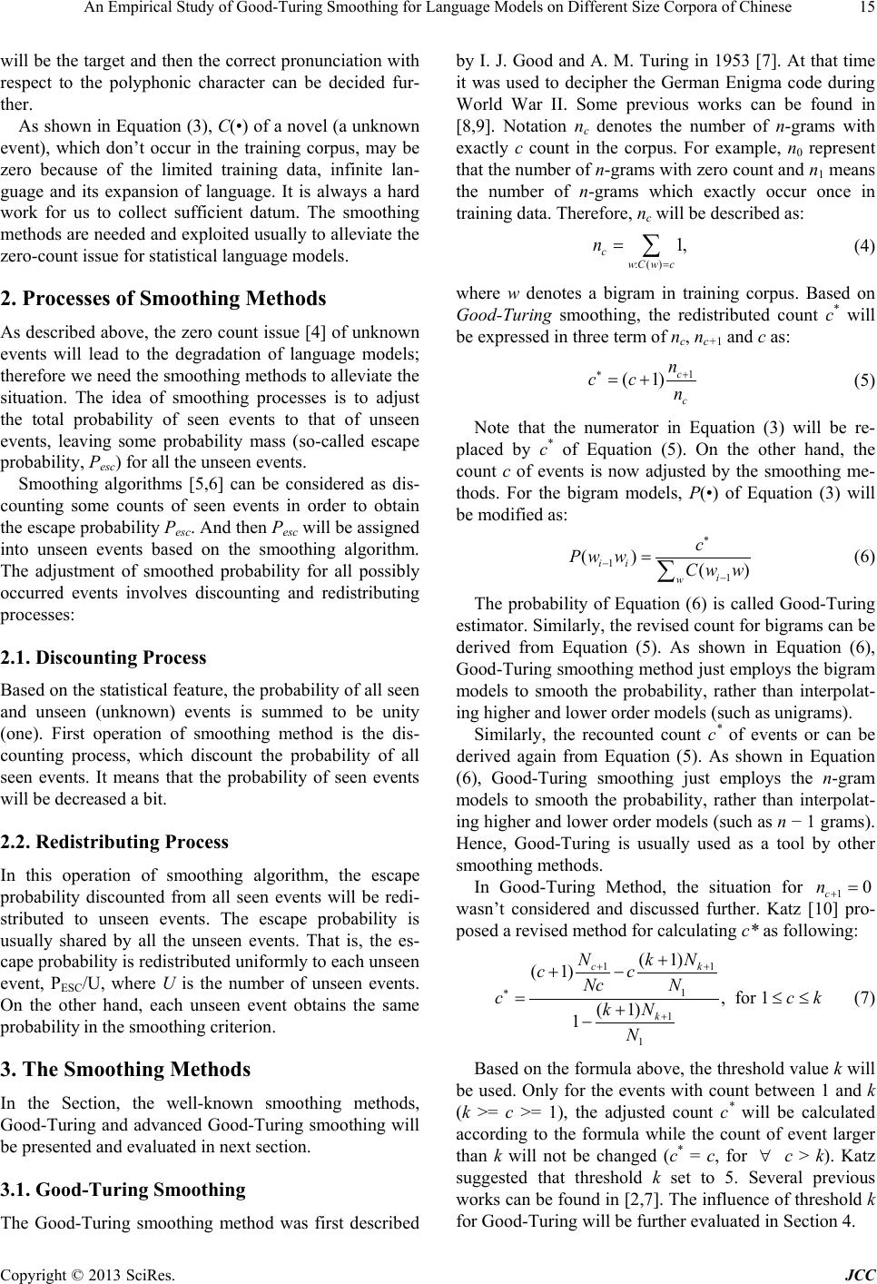

An Empirical Study of Good-Turing Smoothing for Language Models on Different Size Corpora of Chinese

will be the target and then the correct pronunciation with

respect to the polyphonic character can be decided fur-

ther.

As shown in Equation (3), C(•) of a novel (a unknown

event), which don’t occur in the training corpus, may be

zero because of the limited training data, infinite lan-

guage and its expansion of language. It is always a hard

work for us to collect sufficient datum. The smoothing

methods are needed and exploited usually to alleviate the

zero-count issue for statistical language models.

2. Processes of Smoothing Methods

As described above, the zero count issue [4] of unknown

events will lead to the degradation of language models;

therefore we need the smoothing methods to alleviate the

situation. The idea of smoothing processes is to adjust

the total probability of seen events to that of unseen

events, leaving some probability mass (so-called escape

probability, Pesc) for all the unseen events.

Smoothing algorithms [5,6] can be considered as dis-

counting some counts of seen events in order to obtain

the escape probability Pesc. And then Pesc will be assigned

into unseen events based on the smoothing algorithm.

The adjustment of smoothed probability for all possibly

occurred events involves discounting and redistributing

processes:

2.1. Discounting Process

Based on the statistical feature, the probability of all seen

and unseen (unknown) events is summed to be unity

(one). First operation of smoothing method is the dis-

counting process, which discount the probability of all

seen events. It means that the probability of seen events

will be decreased a bit.

2.2. Redistributing Process

In this operation of smoothing algorithm, the escape

probability discounted from all seen events will be redi-

stributed to unseen events. The escape probability is

usually shared by all the unseen events. That is, the es-

cape probability is redistribu ted uniformly to each unseen

event, PESC/U, where U is the number of unseen events.

On the other hand, each unseen event obtains the same

probability in the smoothing criterion.

3. The Smoothing Methods

In the Section, the well-known smoothing methods,

Good-Turing and advanced Good-Turing smoothing will

be presented and evaluated in next section.

3.1. Good-Turing Smoothing

The Good-Turing smoothing method was first described

by I. J. Good and A. M. Turing in 1953 [7]. At that time

it was used to decipher the German Enigma code during

World War II. Some previous works can be found in

[8,9]. Notation nc denotes the number of n-grams with

exactly c count in the corpus. For example, n0 represent

that the number of n-grams with zero count and n1 means

the number of n-grams which exactly occur once in

training data. Therefo re, nc will be described as:

:()

cwC wc

∑

(4)

where w denotes a bigram in training corpus. Based on

Good-Turing smoothing, the redistributed count c* will

be expressed in three term of nc, nc+1 and c as:

(1) c

cc n

∗+

= +

(5)

Note that the numerator in Equation (3) will be re-

placed by c* of Equation (5). On the other hand, the

count c of events is now adjusted by the smoothing me-

thods. For the bigram models, P(•) of Equation (3) will

be modified as:

() ()

ii i

Pw wCw w

∗

−

=∑

(6)

The probability of Equation (6) is called Good-Turing

estimator. Similarly, the revised count for bigrams can be

derived from Equation (5). As shown in Equation (6),

Good-Turing smoothing method just employs the bigram

models to smooth the probability, rather than interpolat-

ing higher and lower order models (such as unigram s).

Similarly, the recounted count c* of events or can be

derived again from Equation (5). As shown in Equation

(6), Good-Turing smoothing just employs the n-gram

models to smooth the probability, rather than interpolat-

ing higher and lower order models (such as n − 1 grams).

Hence, Good-Turing is usually used as a tool by other

smoothing methods.

In Good-Turing Method, the situation for

wasn’t considered and discussed further. Katz [10] pro-

posed a revised method for ca l c ulating c* as following:

( 1)

,for 1

( 1)

N kN

Nc N

c ck

∗

+−

= ≤≤

−

(7)

Based on the formula above, the threshold value k will

be used. Only for the events with count between 1 and k

(k >= c >= 1), the adjusted count c* will be calculated

according to the formula while the count of event larger

than k will not be changed (c* = c, for

∀

c > k). Katz

suggested that threshold k set to 5. Several previous

works can be found in [2,7]. The influence of threshold k

for Good-Turing will be further evaluated in Section 4.

An Empirical Study of Good-Turing Smoothing for Language Models on Different Size Corpora of Chinese

3.2. Advanced Issues of Good-Turing Method

Good-Turing smoothing has been employed in many

natural language applications. Previous works [3,11,12]

discussed the related parameters, such as cut-off k in

Good-Turing method. However, these works employ

English corpus only. In this section, w e will focus on the

Good-Turing method in Mandarin corpus and further

analyze the problems of Good-Turing for Chinese corpus

with various siz e, a n d differe nt cut-off value k.

As shown in Equation (8), Good-Turing reestimate

count c* of all events in term of original count c and

event number nc and nc+1. In practice, the discounted

count c* is not used for all count c. Assumed that larger

counts c are always much reliable. Recount c* are set by

Katz [5], in which c denotes the count of an event, c*

denotes the recount of an event, suggeste d by Katz ,1987

for English data. ni denotes the number of bigrms with i

counts, k denotes the cut-off value.

Good-Turing was first applied as a smoothing method

for n-gram models by Katz [5]. Until now, few papers

discuss the related problems between cut-off k and en-

tropy for Mandarin corpus, even for English. Katz sug-

gested a cut-off k at 5 as threshold for English corpus.

Another important parameter of Good-Turing is the best

kb (not ever discussed in previous works) in term of

training size N.

For Chinese character unigram model, we first calcu-

late the recount c* (c >= 0). Referring to the empirical

results, some recounts c* are negative (<0). In such case,

furthermore it leads to negative probability P and vi-

olates the statistical principle. For instance, c = 8, n8 =

106, n9 = 67, k = 10, the recount c* can be calculated and

is negative −20.56.

3.3. Models Evaluation-Cross Entropy and

Perplexity

Two commonly used schemes for evaluaitng the quality

of language model LM are referred to the entropy and

perplexity [13,14]. Supposed that a sample T is consisted

of sev eral ev ents e1, e2, …, em of m string s. The probabil-

ity P for a given testing sample T is calculated as fol-

lowing:

() ()

PT Pe

∏

(9)

where

)(

is the probability for the event ei, and

)(TE

can be regarded as the coded length for all events

in testing datasets:

()( )log( )()log()

ETPx PxPePe

=−=−

∑∑

(10)

()

() 2

PP T=

(11)

where E(T) and PP(T) denote the entropy (log model

probability) and perplexity for testing dataset T respec-

tively. Emin stands for the minimum entropy for a mode l.

The perplexity PP is usually regarded as the average

number for selected number which will be the possible

candidates referred to a known sequence. When a lan-

guage model is employed to predict the next appearing

word in the curr ent given context, the perplexity is adop-

ted to compare and evaluate n-gram statistical language

models.

In general, lower entropy E leads to lower PP for the

language models. It means that the lower PP, the better

performance of language models. Therefore, perplexity is

a quality measurement for LM. While two language mo-

dels, LM1 and LM2, are compared, the one with lower

perplexity is the better language representation and com-

monly provides higher performance.

In fact, the p robab ility d istributio n fo r t esting language

models is usually unknown. The cross entropy (CE) is

another measure for evaluating a language model. The

model which can predict better the next occurring event

always achieves lower cross entropy. In general situation,

ECE >=

, E denotes the entropy using the same language

model M for training and testing models. The Cross En-

tropy can be expressed as:

123 123

(, )

lim(... )log(...)

nWL

CEp M

pwww wMwww w

→∞ ∈

=∑

(12)

Based on the Shannon-McMillan-Breiman theorem [7],

formula 12 can be simplified as following:

123

( ,)limlog(...)

CEpMMwwww

→∞

(13)

4. Experiments and Evaluation

Chinese Giga Word (CGW) is the Chinese corpus col-

lected from several world news databases and issued by

Linguistic Data Consortium (LDC). In the paper, we

adopted the CGW 3.0 of newest version published on

September 2009. The CGW news sources are Agence

France-Presse, Central News Agency of Taiwan, Xinhua

News Agency of Beijing, aned Zaobao Newspaper of

Singapore.

In the paper, we will cr eate 10 Unigram language mo-

dels with Chinese words for experiments. At first, we

read in random the paper of Chinese words from CGW

corpus, a language model LM1 will be created for the

first 3 × 107 (30 M) Chinese words. In the following, the

other new model LM2 can be created consequently for

the next 3 × 107 Chinese words. In other words, LM2 is

consisted of first 6 × 107 (60 M) Chinese words of CGW,

first half of which is also used to create LM1.

In the paper, the 10 language models created by dif-

ferent size of corpus are evaluated sequentially for inside

An Empirical Study of Good-Turing Smoothing for Language Models on Different Size Corpora of Chinese

testing on these 10 models. As shown in Table 1, the

x-axis and y-axis present the training model (TrM) and

testing models (TeM) respectively. For each row in Ta-

ble 1, testing models are used for evaluating 10 training

models TrM. On the other side, 10 testing models TeM

will be used respectively to evaluate one of 10 training

models for GT smoothing. Figure 1 presents the results

on 3 dimensions respect to Table 1.

The results of perplexity (PP) for Good-Turing smoo-

thing are drawn in Figure 2. Note that the smaller size of

testing models, the lower of perplexity and the larger size

of training models, the higher of perplexity. For each row,

it is apparent that the lowest P P, bold numbers displayed

on the diagonal line in the table, can be achieved on the

same training and testing models. All the results always

match

),()( MpCEpE <=

, as described in Section 3.3.

4.1. Advanced Issues in Good-Turing

As described in Section 3.1, the situation for

wasn’t discussed and processed further by the Good-

Turing Method. Katz [5] proposed a revised method for

Table 1. Perplexity for good-turing smoothing method.

TrM

TeM 30 M

60 M

90 M

120

M 150

M 180

M 210

M 240

M 270

M 300

test 30 M 4013 4103

4177

4237 4290 4339 4384 4426

4472

4512

test 60 M 4211 4063

4110

4156 4202 4246 4286 4325

4368

4406

test 90 M 4490 4293

4214

4243 4280 4317 4352 4387

4426

4462

test 120 M 4710 4491

4379

4337 4359 4388 4418 4449

4484

4518

test 150 M 4923 4691

4556

4490 4459 4477 4501 4528

4560

4591

test 180 M 5125 4882

4732

4650 4600 4575 4591 4613

4641

4669

test 210 M 5294 5044

4882

4790 4730 4689 4670 4684

4707

4732

test 240 M 5459 5202

5030

4930 4862 4810 4773 4754

4769

4789

test 270 M 5651 5385

5201

5091 5015 4953 4903 4868

4845

4858

test 300 M 5834 5562

5368

5250 5166 5097 5036 4990

4951

4933

Avg. 4971 4771

4665

4618 4596 4589 4591 4602

4622

4647

Figure 1. PP results display on 3 dimensions with respect to

Table 2 for GT smoothing.

Figure 2. Results of perplexity PP of Good-Turing.

calculating c* based on Equation (7). It is obvious that

Good-Turing (GT) smoothing is always superior to the

advanced Good-Turing (AGT) for all the testing models.

On the other hands, the AGT set the thresholds k (k = 5)

and avoid the issue caused by the situation

n+=

while it will lead to the degradation of performance (hi-

gher perpl exity) for all training models.

Figure 3 presents the results of perplexity PP of

Good-Turing smoothing. Comparison for Good-Turing

and Advanced Good-Turing smoothing are displayed in

Figure 4. It is obvious that the GT is always superior to

that of AGT for all 10 TrM models. Our observation is

the setting for cut off k proposed by KATZ for Good-

Turing smoothing can’t achieve better performance while

it avoided occurrence of situation, which will lead to

violation of probability.

Comparison for Good-Turing (GT) and Advanced

Good-Turing (AGT) smoothing are displayed in Figure

4. It is obvious that the GT is always superior to that of

AGT for all 10 TrM models. In Figure 4, two observa-

tions are the same as described for GT and AGT

smoothing:

1) the low est PP was achieved on TrM120M, for av e r ag e

PP of lower triangle of each training models.

2) the lowest PP was also achieved on the model

TrM180M and TrM210M, for average PP of each training

models. The perplexity for TrM with size larg er than 180

M words will be also gradually increased.

Based on the evaluation results of PP for three smooth-

ing methods, we could conclude that, in general case for

average perplexity, the lowest PP can be achieved on

model TrM120M. The experiment results could prove that

the model which was created on larger than 180 M cor-

pus can’t achieve a better performance. On the other

hand, our experiments supported that the model with

middle size of corpus of 180 M Chinese words can al-

ways achieve the best performance of language model.

4.2. Evaluation of Outside Testing

In the following experiments, the text sources from

ASBC corpus are exploited as outside datasets. The

test3 0 M

test120M

test210M

test300M

3800

4300

4800

5300

5800

30M

60M

90M

120M

150M

180M

210M

240M

270M

300M

test30M

test60M

test90M

test120M

test150M

test180M

test210M

test240M

test270M

test300M

4000.0

4100.0

4200.0

4300.0

4400.0

4500.0

4600.0

4700.0

4800.0

4900.0

5000.0

30M

60M

90M

120M

150M

180M

210M

240M

270M

300M

Avg. perplexity of Good-Turing

lower tri.

total avg.

diagonal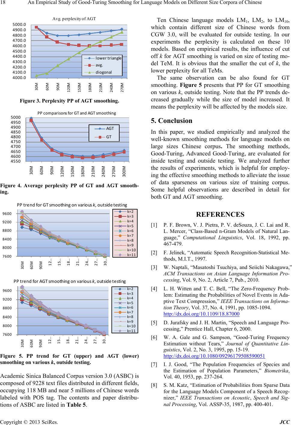

An Empirical Study of Good-Turing Smoothing for Language Models on Different Size Corpora of Chinese

Figure 3. Perplexity PP of AGT smoothing.

Figure 4. Average perplexity PP of GT and AGT smooth-

ing.

Figure 5. PP trend for GT (upper) and AGT (lower)

smoothing on various k, outside testing.

Academic Sinica Balanced Corpus version 3.0 (ASBC) is

compose d of 9228 text files distributed in different fields,

occupying 118 MB and near 5 millions o f Chinese words

labeled with POS tag. The contents and paper distribu-

tions of ASBC are listed in Table 5.

Ten Chinese language models LM1, LM2, to LM10,

which contain different size of Chinese words from

CGW 3.0, will be evaluated for outside testing. In our

experiments the perplexity is calculated on these 10

models. Based on empirical results, the influence of cut

off k for AGT smoothing is varied on size of testing mo -

del TeM. It is obvious that the smaller the cut of k, the

lower perplexity for all TeMs.

The same observation can be also found for GT

smoothing. Figure 5 presents that PP for GT smoothing

on various k, outside testing. Note that the PP trends de-

creased gradually while the size of model increased. It

means the perplexity will be affected by the models size.

5. Conclusion

In this paper, we studied empirically and analyzed the

well-known smoothing methods for language models on

large sizes Chinese corpus. The smoothing methods,

Good-Turing, Advanced Good-Turing, are evaluated for

inside testing and outside testing. We analyzed further

the results of experiments, which is helpful for employ-

ing the effective smoothing methods to alleviate the issu e

of data sparseness on various size of training corpus.

Some helpful observations are described in detail for

both GT an d AGT smoot hing.

REFERENCES

[1] P. F. Brown, V. J. Pietra, P. V. deSouza, J. C. Lai and R.

L. Mercer, “Class-Based n-Gram Models of Natural Lan-

guage,” Computational Linguistics, Vol. 18, 1992, pp.

467-479.

[2] F. Jelinek, “Automatic Speech Recognition-Statistical Me-

thods, M.I.T., 1997.

[3] W. Naptali, “Masatoshi Tsuchiya, and Seiichi Nakagawa,”

ACM Transactions on Asian Language Information Pro-

cessing, Vol. 9, No. 2, Article 7, Pub., 2010.

[4] L. H. Witten and T. C. Bell, “The Zero-Frequency Prob-

lem: Estimating the Probabilities of Novel Eve nts in Ada-

ptive Text Compression,” IEEE Transactions on Informa-

tion Theory, Vol. 37, No. 4, 1991, pp. 1085-1094.

http://dx.doi.org/10.1109/18.87000

[5] D. Jurafsky and J. H. Martin, “Speech and Language Pro-

cessing,” Prentice Hall, Chapter 6, 2000.

[6] W. A. Gale and G. Sampson, “Good-Turing Frequency

Estimation without Tears,” Journal of Quantitative Lin-

guistics, Vol. 2, No. 3, 1995, pp. 15-19.

http://dx.doi.org/10.1080/09296179508590051

[7] I. J. Good, “The Population Frequencies of Species and

the Estimation of Population Parameters,” Biometrika,

Vol. 40, 1953, pp. 237-264.

[8] S. M. Katz, “Estimation of Probabilities from Sparse Data

for the Language Models Component of a Speech Recog-

nizer,” IEEE Transactions on Acoustic, Speech and Sig-

nal Processing, Vol. ASSP-35, 1987, pp. 400-401.

4000.0

4100.0

4200.0

4300.0

4400.0

4500.0

4600.0

4700.0

4800.0

4900.0

5000.0

30M

60M

90M

120M

150M

180M

210M

240M

270M

A vg . pe rpl exi t y of A GT

lower triangle

avg.

diogonal

4550

4600

4650

4700

4750

4800

4850

4900

4950

5000

30M

60M

90M

120M

150M

180M

210M

240M

270M

300M

AGT

PP comparisons for GT and AGT smoothing

7600

8000

8400

8800

9200

9600

30M

60M

90M

12…

15…

18…

21…

24…

27…

30…

k=2

k=3

k=4

k=5

k=6

k=7

k=8

k=9

k=10

k=11

PP trend for GT smoothing on various k, outside testing

7600

8000

8400

8800

9200

9600

30M

60M

90M

12…

15…

18…

21…

24…

27…

30…

k=2

k=3

k=4

k=5

k=6

k=7

k=8

k=9

k=10

k=11

PP trend for AGT smoothing on various k, outside testing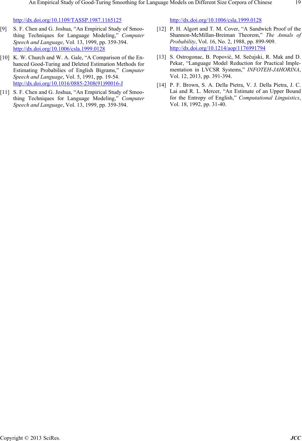

An Empirical Study of Good-Turing Smoothing for Language Models on Different Size Corpora of Chinese

http://dx.doi.org/10.1109/TASSP.1987.1165125

[9] S. F. Chen and G. Joshua, “An Empirical Study of Smoo-

thing Techniques for Language Modeling,” Computer

Speech and Language, Vol. 13, 1999, pp. 359-394.

http://dx.doi.org/10.1006/csla.1999.0128

[10] K. W. Church and W. A. Gale, “A Comparison of the En-

hanced Good-Turing and Deleted Estimation Methods for

Estimating Probabilies of English Bigrams,” Computer

Speech and Language, Vol. 5, 1991, pp. 19-54.

http://dx.doi.org/10.1016/0885-2308(91)90016-J

[11] S. F. Chen and G. Joshua, “An Empirical Study of Smoo-

thing Techniques for Language Modeling,” Computer

Speech and Language, Vol. 13, 1999, pp. 359-394.

http://dx.doi.org/10.1006/csla.1999.0128

[12] P. H. Algort and T. M. Cover, “A Sandwich Proof of the

Shannon-McMillan-Breiman Theorem,” The Annals of

Probability, Vol. 16, No. 2, 1988, pp. 899-909.

http://dx.doi.org/10.1214/aop/1176991794

[13] S. Ostrogonac, B. Popović, M. Sečujski, R. M ak and D.

Pekar, “Language Model Reduction for Practical Imple-

mentation in LVCSR Systems,” INFOTEH-JAHORINA,

Vol. 12, 2013, pp. 391-394.

[14] P. F. Brown, S. A. Della Pietra, V. J. Della Pietra, J. C.

Lai and R. L. Mercer, “An Estimate of an Upper Bound

for the Entropy of English,” Computational Linguistics,

Vol. 18, 1992, pp. 31-40.