Application of Soft Computing Methods in Predicting Evapotranspiration

doi:10.4236/ojg.2013.37045

Paper Menu >>

Journal Menu >>

Open Journal of Geology, 2013, 3, 397-403

Published Online November 2013 (http://www.scirp.org/journal/ojg)

http://dx.doi.org/10.4236/ojg.2013.37045

Open Access OJG

Application of Soft Computing Methods

in Predicting Evapotranspiration

Afshin Honarbakhsh1, Mostafa Moradi Dashtpagerdi2*, Hassan Vagharfard3

1Faculty of Natural Resources and Earth Sciences, University of Shahrekord, Shahrekord, Iran

2Graduated Watershed Management, Organization of Natural Resources and Watershed Management,

Karoon Watershed Management Office (KWMO), Shahrekord, Iran

3Faculty of Natural Resources, Hormozgan University, Bandarabbas, Iran

Email: *[email protected]

Received May 21, 2013; revised June 20, 2013; accepted June 28, 2013

cense, which permits unrestricted use, distribution, and reproduction in any medium, provided the original work is properly cited.

ABSTRACT

Exact prediction of evapotranspiration is necessary for study, design and management of irrigation systems. In this re-

search, the suitability of soft computing approaches namely, fuzzy rule base, fuzzy regression and artificial neural net-

works for estimation of daily evapotranspiration has been examined and the results are compared to real data measured

by lysimeter on the basis of reference crop (grass). Using daily climatic data from Haji Abad station in Hormozgan,

west of Iran, including maximum and minimum temperatures, maximum and minimum relative humidities, wind sp eed

and sunny hours, evapotranspiration was predicted by soft computing methods. The predicted evapotranspiration values

from fuzzy rule base, fuzzy linear regression and artificial neural networks show root mean square error (RMSE) of

0.75, 0.79 and 0.81 mm/day and coefficient of determination of (R2) of 0.90, 0.87 and 0.85, respectively. Therefore,

fuzzy rule base approach was found to be the most appropriate method employed for estimating evapotranspiration.

Keywords: Evapotranspiration; Fuzzy Rule Base; Fuzzy Regression; Artificial Neural Network

1. Introduction

Evapotranspiration is one of the most important factors

in agriculture and the hydrological cycle that can be in-

fluenced by global warming and climatic changes [1].

The process of evapotranspiration (ET) is an important

part of the water cycle and exactly estimating the value

of ET is necessary for designing irrigation systems and

water resources management. Accurate estimation of ET

is crucial in agriculture. This is due to the fact that its

over-estimation causes waste of valuable water resources

and its underestimation leads to the plant moisture stress

and decrease in the crop yield. Prediction methods de-

veloped over the past few decades range from simple

ones such as Blany-Criddle to complex ones which use

physical processes like Penman compound method [2].

Penman approach used parameters such as dynamic of

evaporation, intensity of net radiations and surface aero-

dynamic characteristics. Montieth et al. (1965) later im-

proved this method by considering the plant daily resis-

tance and Penman-Montieth equation [3]. Several re-

searchers studied validation of these equations [4,5].

Jenson et al. (1990) compared results of twenty of such

methods with the results of lysimeters in 11 stations lo-

cated in different parts of the world with various climates

and concluded that in all climates the Penman-Montieth

method gave the best results [6]. In recent years, soft

computing methods including fuzzy rule base model

(FRBM), artificial neural Networks (ANN) and also a

combination of them have been employed for estimating

ET.

Burton et al. (2000) used ANNs and estimated daily

evaporation from pan evaporation by 2044 data gathered

from various places all over the world from 1992 to 1996

[7]. Input data were precipitation, temperature, relative

humidity, solar irradiance and wind speed. Compared

with multiple linear regressions methods such as the one

proposed by Priestley-Taylor (1972), ANN provided the

minimum error of 1.11 mm/day in ET estimation [8].

Odhiambo et al. (2001) compared the results from

FRBM with those of Penman-Montieth [9] and Sha-

yannejad et al. (2007 ) used Fuzzy linear regression (FLR)

for ET estimation in Hamadan, Iran and demonstrated

*Corresponding a uthor.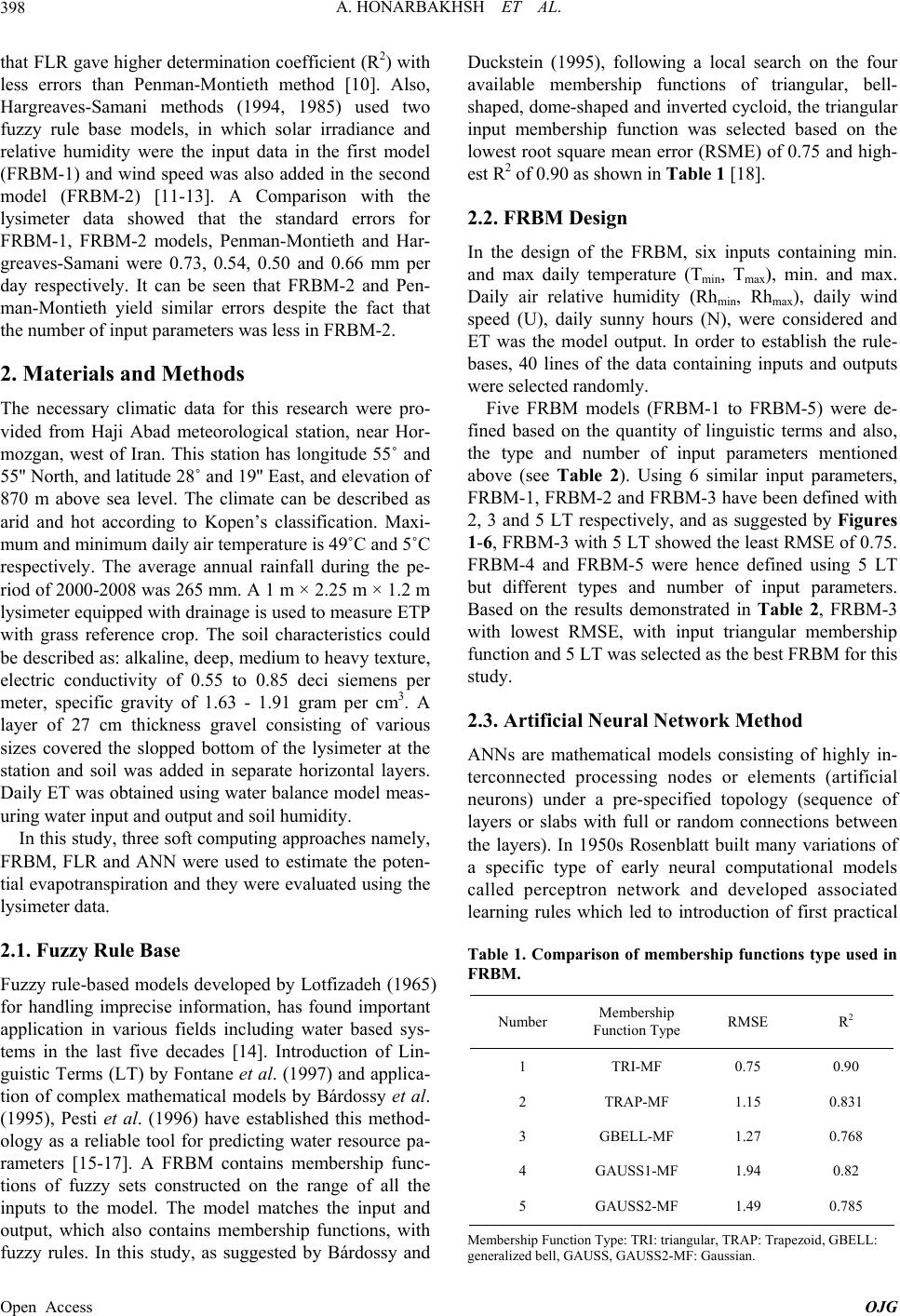

A. HONARBAKHSH ET AL.

398

that FLR gave higher determination coefficient (R2) with

less errors than Penman-Montieth method [10]. Also,

Hargreaves-Samani methods (1994, 1985) used two

fuzzy rule base models, in which solar irradiance and

relative humidity were the input data in the first model

(FRBM-1) and wind speed was also added in the second

model (FRBM-2) [11-13]. A Comparison with the

lysimeter data showed that the standard errors for

FRBM-1, FRBM-2 models, Penman-Montieth and Har-

greaves-Samani were 0.73, 0.54, 0.50 and 0.66 mm per

day respectively. It can be seen that FRBM-2 and Pen-

man-Montieth yield similar errors despite the fact that

the number of input parameters was less in FRBM-2.

2. Materials and Methods

The necessary climatic data for this research were pro-

vided from Haji Abad meteorological station, near Hor-

mozgan, west of Iran. This station has longitude 55˚ and

55'' Nort h, and latitude 28˚ and 19'' East, and elev ation of

870 m above sea level. The climate can be described as

arid and hot according to Kopen’s classification. Maxi-

mum and minimum daily air temperature is 49˚C and 5˚C

respectively. The average annual rainfall during the pe-

riod of 2000-2008 was 265 mm. A 1 m × 2.25 m × 1.2 m

lysimeter equipped with drainage is used to measure ETP

with grass reference crop. The soil characteristics could

be described as: alkaline, deep, medium to heavy texture,

electric conductivity of 0.55 to 0.85 deci siemens per

meter, specific gravity of 1.63 - 1.91 gram per cm3. A

layer of 27 cm thickness gravel consisting of various

sizes covered the slopped bottom of the lysimeter at the

station and soil was added in separate horizontal layers.

Daily ET was obtained using water balance model meas-

uring water input and output and soil humidity.

In this study, three soft computing approaches namely,

FRBM, FLR and ANN were used to estimate the poten-

tial evapotranspiration and they were evaluated using the

lysimeter data.

2.1. Fuzzy Rule Base

Fuzzy rule-based models developed by Lotfizadeh (1965)

for handling imprecise information, has found important

application in various fields including water based sys-

tems in the last five decades [14]. Introduction of Lin-

guistic Terms (LT) by Fontane et al. (1997) and applica-

tion of complex mathematical models by Bárdossy et al.

(1995), Pesti et al. (1996) have established this method-

ology as a reliable tool for predicting water resource pa-

rameters [15-17]. A FRBM contains membership func-

tions of fuzzy sets constructed on the range of all the

inputs to the model. The model matches the input and

output, which also contains membership functions, with

fuzzy rules. In this study, as suggested by Bárdossy and

Duckstein (1995), following a local search on the four

available membership functions of triangular, bell-

shaped, dome-shaped and inverted cycloid, the triangular

input membership function was selected based on the

lowest root square mean error (RSME) of 0.75 and high-

est R2 of 0.90 as shown in Tabl e 1 [18].

2.2. FRBM Design

In the design of the FRBM, six inputs containing min.

and max daily temperature (Tmin, Tma x), min. and max.

Daily air relative humidity (Rhmin, Rhmax), daily wind

speed (U), daily sunny hours (N), were considered and

ET was the model output. In order to establish the rule-

bases, 40 lines of the data containing inputs and outputs

were selected randomly.

Five FRBM models (FRBM-1 to FRBM-5) were de-

fined based on the quantity of linguistic terms and also,

the type and number of input parameters mentioned

above (see Table 2). Using 6 similar input parameters,

FRBM-1, FRBM-2 and FRBM-3 have been defined with

2, 3 and 5 LT respectively, and as suggested by Figures

1-6, FRBM-3 with 5 LT showed the least RMSE of 0.75.

FRBM-4 and FRBM-5 were hence defined using 5 LT

but different types and number of input parameters.

Based on the results demonstrated in Table 2, FRBM-3

with lowest RMSE, with input triangular membership

function and 5 LT was selected as the best FRBM for this

study.

2.3. Artificial Neural Network Method

ANNs are mathematical models consisting of highly in-

terconnected processing nodes or elements (artificial

neurons) under a pre-specified topology (sequence of

layers or slabs with full or random connections between

the layers). In 1950s Rosenblatt built many variations of

a specific type of early neural computational models

called perceptron network and developed associated

learning rules which led to introduction of first practical

Table 1. Comparison of membership functions type used in

FRBM.

Number Membership

Function Type RMSE R2

1 TRI-MF 0.75 0.90

2 TRAP-MF 1.15 0.831

3 GBELL-MF 1.27 0.768

4 GAUSS1-MF 1.94 0.82

5 GAUSS2-MF 1.49 0.785

Membership Function Type: TRI: triangular, TRAP: Trapezoid, GBELL:

generaliz ed bell, GAUSS, GAUSS2-MF: Gaussian.

Open Access OJG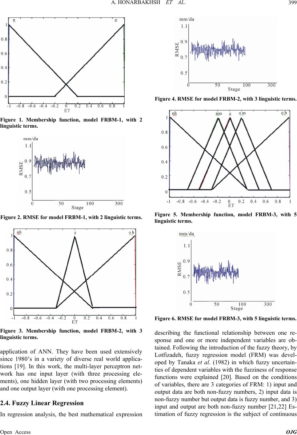

A. HONARBAKHSH ET AL. 399

Figure 1. Membership function, model FRBM-1, with 2

linguistic terms.

Figure 2. RMSE for model FRBM-1, with 2 linguistic terms.

Figure 3. Membership function, model FRBM-2, with 3

linguistic terms.

application of ANN. They have been used extensively

since 1980’s in a variety of diverse real world applica-

tions [19]. In this work, the multi-layer perceptron net-

work has one input layer (with three processing ele-

ments), one hidden layer (with two processing elements)

and one output layer (with one processing element).

2.4. Fuzzy Linear Regression

In regression analysis, the best mathematical expression

Figure 4. RMSE for model FRBM-2, with 3 linguistic terms.

Figure 5. Membership function, model FRBM-3, with 5

linguistic terms.

Figure 6. RMSE for model FRBM-3, with 5 linguistic terms.

describing the functional relationship between one re-

sponse and one or more independent variables are ob-

tained. Following the introduction of the fuzzy theory, by

Lotfizadeh, fuzzy regression model (FRM) was devel-

oped by Tanaka et al. (1982) in which fuzzy uncertain-

ties of dependent variables with the fuzziness of response

functions were explained [20]. Based on the conditions

of variables, there are 3 categories of FRM: 1) input and

output data are both non-fuzzy numbers, 2) input data is

non - f uzzy nu mber but output data is fuzzy number, and 3)

input and output are both non-fuzzy number [21,22] Es-

timation of fuzzy regression is the subject of continuous

Open Access OJG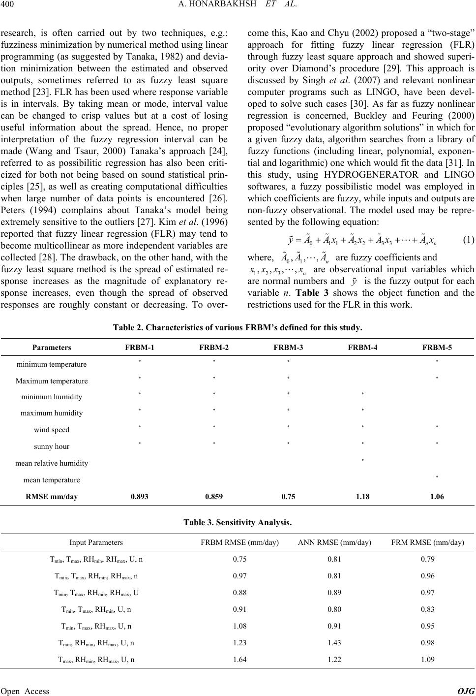

A. HONARBAKHSH ET AL.

Open Access OJG

400

come this, Kao and Chyu (200 2) proposed a “two-stage”

approach for fitting fuzzy linear regression (FLR)

through fuzzy least square approach and showed superi-

ority over Diamond’s procedure [29]. This approach is

discussed by Singh et al. (2007) and relevant nonlinear

computer programs such as LINGO, have been devel-

oped to solve such cases [30]. As far as fuzzy nonlinear

regression is concerned, Buckley and Feuring (2000)

proposed “evolutionary algorithm solutions” in which for

a given fuzzy data, algorithm searches from a library of

fuzzy functions (including linear, polynomial, exponen-

tial and logarithmic) one which would fit the data [31]. In

this study, using HYDROGENERATOR and LINGO

softwares, a fuzzy possibilistic model was employed in

which coefficients are fuzzy, while inputs and outputs are

non-fuzzy observational. The model used may be repre-

sented by the following equation:

research, is often carried out by two techniques, e.g.:

fuzziness minimization by numerical method using linear

programming (as suggested by Tanaka, 1982) and devia-

tion minimization between the estimated and observed

outputs, sometimes referred to as fuzzy least square

method [23]. FLR has been used where response variable

is in intervals. By taking mean or mode, interval value

can be changed to crisp values but at a cost of losing

useful information about the spread. Hence, no proper

interpretation of the fuzzy regression interval can be

made (Wang and Tsaur, 2000) Tanaka’s approach [24],

referred to as possibilitic regression has also been criti-

cized for both not being based on sound statistical prin-

ciples [25], as well as creating computational difficulties

when large number of data points is encountered [26].

Peters (1994) complains about Tanaka’s model being

extremely sensitive to the outliers [27]. Kim et al. (199 6)

reported that fuzzy linear regression (FLR) may tend to

become multicollinear as more independ ent variables are

collected [28]. The drawback, on the other hand, with the

fuzzy least square method is the spread of estimated re-

sponse increases as the magnitude of explanatory re-

sponse increases, even though the spread of observed

responses are roughly constant or decreasing. To over-

0112233nn

AAxAxAxAx 

 

 (1)

where, 01

,,,

 



are fuzzy coefficients and

123

xx x are observational input variables which

are normal numbers and

 is the fuzzy output for each

variable n. Table 3 shows the object function and the

restrictions used for the FLR in this work.

Table 2. Characteristics of various FRBM’s de fined for this study.

Parameters FRBM-1 FRBM-2 FRBM-3 FRBM-4 FRBM-5

minimum temperature * * * *

Maximum temperature * * * *

minimum humidity * * * *

maximum humidity * * * *

wind speed * * * * *

sunny hour * * * * *

mean relative humidity *

mean temperature *

RMSE mm/day

0.893 0.859

0.75 1.18 1.06

Table 3. Sensitivity Analysis.

Input Parameters FRBM RMSE (mm/day) ANN RMSE (mm/day) FRM RMSE (mm/day)

Tmin, Tmax, RHmin , RHmax, U, n 0.75 0.81 0.79

Tmin, Tmax, RHmin , RHmax, n 0.97 0.81 0.96

Tmin, Tmax, RHmin , RHmax, U 0.88 0.89 0.97

Tmin, Tmax, RHmin , U, n 0.91 0.80 0.83

Tmin, Tmax, RHmax , U, n 1.08 0.91 0.95

Tmin, RHmin, RHma x, U, n 1.23 1.43 0.98

Tmax, RHmin, RHmax, U, n 1.64 1.22 1.09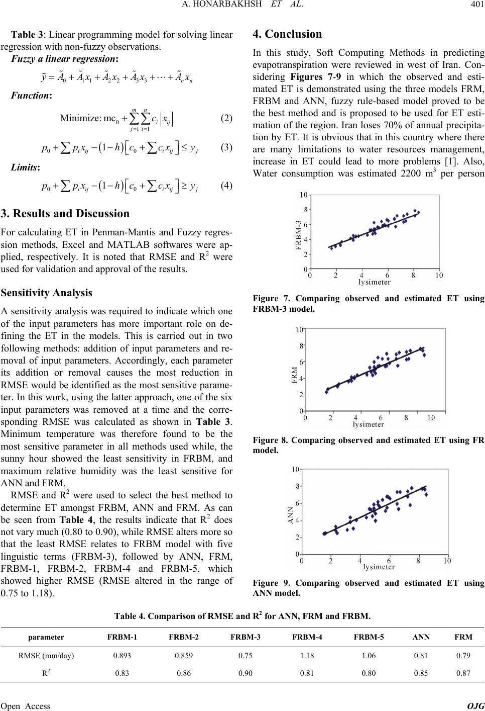

A. HONARBAKHSH ET AL. 401

Table 3: Liodel for solving linear near programming m

regression with non-fuzzy observations.

Fuzzy a linear regression:

0112233nn

AAxAx 

 

Ax Ax

 



Function:

011

Minimize: mcmn

iij



 (2)

y (3)

Limits:

y (4)

3. Results and Discussion

antis and Fuzzy regres-

as required to indicate which one

ft Computing Methods in predicting



iijiij j

ppx hccx



 







iijiij j

ppx hccx



 





For calculating ET in Penman-M

sion methods, Excel and MATLAB softwares were ap-

plied, respectively. It is noted that RMSE and R2 were

used for validation and approval of the results.

Sensitivity Analysis

A sensitivity analysis w

of the input parameters has more important role on de-

fining the ET in the models. This is carried out in two

following methods: addition of input parameters and re-

moval of input parameters. Accordingly, each parameter

its addition or removal causes the most reduction in

RMSE would be identified as the most sensitive parame-

ter. In this work, using the latter approach, one of the six

input parameters was removed at a time and the corre-

sponding RMSE was calculated as shown in Tab le 3.

Minimum temperature was therefore found to be the

most sensitive parameter in all methods used while, the

sunny hour showed the least sensitivity in FRBM, and

maximum relative humidity was the least sensitive for

ANN and FRM.

RMSE and R2 were used to select the best method to

determine ET amongst FRBM, ANN and FRM. As can

be seen from Table 4, the results indicate that R2 does

not vary much (0.80 to 0.90), while RMSE alters more so

that the least RMSE relates to FRBM model with five

linguistic terms (FRBM-3), followed by ANN, FRM,

FRBM-1, FRBM-2, FRBM-4 and FRBM-5, which

showed higher RMSE (RMSE altered in the range of

0.75 to 1.18).

4. Conclusion

In this study, So

evapotranspiration were reviewed in west of Iran. Con-

sidering Figures 7-9 in which the observed and esti-

mated ET is demonstrated using the three models FRM,

FRBM and ANN, fuzzy rule-based model proved to be

the best method and is proposed to be used for ET esti-

mation of the region. Ir an loses 70% of annu al precipita-

tion by ET. It is obvious that in this country where there

are many limitations to water resources management,

increase in ET could lead to more problems [1]. Also,

Water consumption was estimated 2200 m3 per person

Figure 7. Comparing observed and estimated ET using

FRBM-3 model.

Figure 8. Comparing observed and estimated ET using FR

model.

Figure 9. Comparing observed and estimated ET using

Table 4. Comparison of RMSE andRM and FRBM.

parameter F-5 ANN FRM

ANN model.

R2 for ANN, F

RBM-1 FRBM-2 FRBM-3 FRBM-4 FRBM

RMy) SE (mm/da 0.893 0.859 0.75 1.18 1.06 0.81 0.79

R2 0.83 0.86 0.90 0.81 0.80 0.85 0.87

Open Access OJG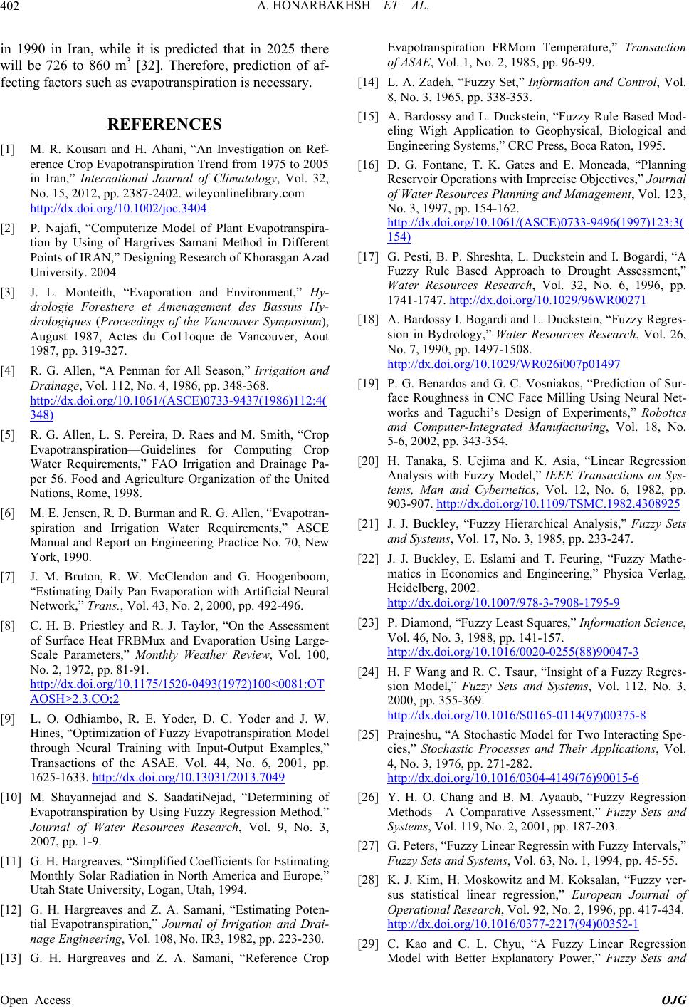

A. HONARBAKHSH ET AL.

402

in 1hile it isicted that25 there

will be 726 to 860 m3 [32]. Therefore, prediction of af-

cting fac such as evappiration isssary.

[1] M. R. Kousari and H. Ahani, “An Investigation on Ref-

erence Crop Efrom 1975 to 2005

in Iran,” Inter matology, Vol. 32,

990 in Iran, w pred in 20

fe torsotrans nece

REFERENCES

vapotranspiration Trend

national Journal of Cli

No. 15, 2012, pp. 2387-2402. wileyonlinelibrary.com

http://dx.doi.org/10.1002/joc.3404

[2] P. Najafi, “Computerize Model of Plant Evapotranspira-

tion by Using of Hargrives Samani Method in Differen

Points of IRAN,” Designing Researt

ch of Khorasgan Azad

eedings of the Vancouver Symposium),

061/(ASCE)0733-9437(1986)112:4(

University. 2004

[3] J. L. Monteith, “Evaporation and Environment,” Hy-

drologie Forestiere et Amenagement des Bassins Hy-

drologiques (Proc

August 1987, Actes du Co11oque de Vancouver, Aout

1987, pp. 319-327.

[4] R. G. Allen, “A Penman for All Season,” Irrigation and

Drainage, Vol. 112, No. 4, 1986, pp. 348-368.

http://dx.doi.org/10.1

348)

[5] R. G. Allen, L. S. Pereira, D. Raes and M. Smit

Evapotranspiration—Guidelines for Computing Crop

Water

h, “

Requirements,” FAO Irrigation and Drainage Pa-

Engineering Practice No. 70, New

ans., Vol. 43, No. 2, 2000, pp. 492-496.

Crop

per 56. Food and Agriculture Organization of the United

Nations, Rome, 1998.

[6] M. E. Jensen, R. D. Burman and R. G. Allen, “Evapotran-

spiration and Irrigation Water Requirements,” ASCE

Manual and Report on

York, 1990.

[7] J. M. Bruton, R. W. McClendon and G. Hoogenboom,

“Estimating Daily Pan Evaporation with Artificial Neural

Network,” Tr

[8] C. H. B. Priestley and R. J. Taylor, “On the Assessment

of Surface Heat FRBMux and Evaporation Using Large-

Scale Parameters,” Monthly Weather Review, Vol. 100,

No. 2, 1972, pp. 81-91.

http://dx.doi.org/10.1175/1520-0493(1972)100<0081:OT

AOSH>2.3.CO;2

[9] L. O. Odhiambo, R. E.

Hines, “Optimization of Fuzzy Evapotranspiration Model

through Neural T

Yoder, D. C. Yoder and J. W.

raining with Input-Output Examples,”

Transactions of the ASAE. Vol. 44, No. 6, 2001, pp.

1625-1633. http://dx.doi.org/10.13031/2013.7049

[10] M. Shayannejad and S. SaadatiNejad, “Determining of

Evapotranspiration by Using Fuzzy Regression Method,”

Journal of Water Resources Research, Vol. 9, No. 3,

ersity, Logan, Utah, 1994.

[13] G. H. Hargreaves and Z. A. Samani, “Reference Crop

Evapoiration FRTemper” Tra on

of ASAE, 1985, pp. 96-99.

4] L. A. Z, “Fuzzy Seformatio Contol.

ives,” Journal

2007, pp. 1-9.

[11] G. H. Hargreaves, “Simplified Coefficients for Estimating

Monthly Solar Radiation in North America and Europe,”

Utah State Univ

[12] G. H. Hargreaves and Z. A. Samani, “Estimating Poten-

tial Evapotranspiration,” Journal of Irrigation and Drai-

nage Engineering, Vol. 108, No. IR3, 1982, pp. 223-230.

transp

, Vol. 1, No. 2Mom ature,nsacti

[1 adeh t,” Inn androl, V

8, No. 3, 1965, pp. 338-353.

[15] A. Bardossy and L. Duckstein, “Fuzzy Rule Based Mod-

eling Wigh Application to Geophysical, Biological and

Engineering Systems,” CRC Press, Boca Raton, 1995.

[16] D. G. Fontane, T. K. Gates and E. Moncada, “Planning

Reservoir Operations with Imprecise Object

of Water Resources Planning and Management, Vol. 123,

No. 3, 1997, pp. 154-162.

http://dx.doi.org/10.1061/(ASCE)0733-9496(1997)123:3(

154)

[17] G. Pesti, B. P. Shreshta, L. Duckstein and I. Bogardi, “A

Fuzzy Rule Based Approach to Drought Assessment,”

Water Resources Research, Vol. 32, No. 6, 1996, pp.

1741-1747. http://dx.doi.org/10.1029/96WR00271

[18] A. Bardossy I. Bogardi and

sion in Bydrology,” Water Resources Research, Vol. 26,

No. 7,

L. Duckstein, “Fuzzy Regres-

1990, pp. 1497-1508.

http://dx.doi.org/10.1029/WR026i007p01497

[19] P. G. Benardos and G. C. Vosniakos, “Prediction of Sur-

face Roughness in CNC Face Milling Using Neural Net-

works and Taguchi’s Design of Experiments,” Robotics

Asia, “Linear Regression

ons on Sys-

and Computer-Integrated Manufacturing, Vol. 18, No.

5-6, 2002, pp. 343-354.

[20] H. Tanaka, S. Uejima and K.

Analysis with Fuzzy Model,” IEEE Transacti

tems, Man and Cybernetics, Vol. 12, No. 6, 1982, pp.

903-907. http://dx.doi.org/10.1109/TSMC.1982.4308925

[21] J. J. Buckley, “Fuzzy Hierarchical Analysis,” Fuzzy Sets

and Systems, Vol. 17, No. 3, 1985, pp. 233-247.

[22] J. J. Buckley, E. Eslami and T. Feuring, “Fuzzy Mathe-

matics in Economics and Engineering,” Physica Verlag,

Heidelberg, 2002.

http://dx.doi.org/10.1007/978-3-7908-1795-9

[23] P. Diamond, “Fuzzy Least Squares,” Information Science,

Vol. 46, No. 3, 1988, pp. 141-157.

http://dx.doi.org/10.1016/0020-0255(88)90047-3

5-8

[24] H. F Wang and R. C. Tsaur, “Insight of a Fuzzy Regres-

sion Model,” Fuzzy Sets and Systems, Vol. 112, No. 3,

2000, pp. 355-369.

http://dx.doi.org/10.1016/S0165-0114(97)0037

ir Applications, Vol.

[25] Prajneshu, “A Stochastic Model for Two Interacting Spe-

cies,” Stochastic Processes and The

4, No. 3, 1976, pp. 271-282.

http://dx.doi.org/10.1016/0304-4149(76)90015-6

[26] Y. H. O. Chang and B. M. Ayaaub, “Fuzzy Regression

Methods—A Comparative Assessment,” Fuzzy Sets and

Systems, Vol. 119, No. 2, 2001, pp. 187-203.

[27] G. Peters, “Fuzzy Li near Re gressi n wit h Fuzzy Inte rvals, ”

Fuzzy Sets and Systems, Vol. 63, No. 1, 1994, pp. 45-55.

[28] K. J. Kim, H. Moskowitz and

sus statistical linear regression,” European Journal of

M. Koksalan, “Fuzzy ver-

Operational Research, Vol. 92, No. 2, 1996, pp. 417-434.

http://dx.doi.org/10.1016/0377-2217(94)00352-1

[29] C. Kao and C. L. Chyu, “A Fuzzy Linear Regression

Model with Better Explanatory Power,” Fuzzy Sets and

Open Access OJG

A. HONARBAKHSH ET AL. 403

Systems, Vol. 126, No. 3, 2002, pp. 401-09.

http://dx.doi.org/10.1016/S0165-0114(01)00069-0

[30] R. K. Singh, Prajneshu and H. Ghosh, “A TWO-Stage

Fizzy Least Squares Procedure for Fitting von Bertalanffy

Growth Model,” 2007.

[31] J. J. Buckey and T. Feuring, “Universal Approximators

for Fuzzy Functions,” Fuzzy Set and Systems, Vol. 113,

No. 3, 2000, pp. 411-415.

[32] A. A. Alesheikh, M. J. Soltani, N. Nouri and M. Khalil-

zadeh, “Land Assessment for Flood Spreading Site Selec-

tion Using Geospatial Information System,” International

Journal of Environmental Science and Technology, Vol. 5,

No. 4, 2008, pp. 455-462.

http://dx.doi.org/10.1007/BF03326041

Open Access OJG