Paper Menu >>
Journal Menu >>
 Energy and Power Engineering, 2013, 5, 1139-1146 doi:10.4236/epe.2013.54B217 Published Online July 2013 (http://www.scirp.org/journal/epe) Model of Three-Phas e Transmission Line with the Theory of Modal Decomposition Implied Rodrigo Cleber da Silva, Sérgio Kurokawa Department of Electrical Engineering, Unesp, Ilha Solteira, Brasil. Email: [email protected], [email protected] Received February, 2013 ABSTRACT This paper shows the development of transmission line model, based on lumped element circuit that provides answers directly in the time and phase domain. This model is valid to represent the ideally transposed line, the phases of each of the small line segments are separated in their modes of propagation and the voltage and current are calculated at the modal domain. However, the conversion phase-mode-phase is inserted in the state equations which describe the currents and voltages along the line of which there is no need to know the user of the model representation of the theory in the line modal domain. Keywords: π-circuits; Electromagnetic Transients; Transmission Lines; Transmission Line Models 1. Introduction It is known that a transmission line power has a basic characteristic that is the fact of their parameters of longitudinal and transverse are distributed along the length of the line. This characteristic with the fact that their parameters of longitudinal line vary as a function of frequency, makes the line of electric power transmission an element with a certain particularities that should be taken into consideration when their representation [1]. The distributed nature of the longitudinal parameters of a transmission line must be taken into account, especially in studies and simulations of transient electromagnetic resulting from operations of maneuvers and atmospheric discharges occurring in the line or around to it. In these situations, the transient current and voltage of the line assume characteristics such that a full understanding of the same is only possible if these quantities are treated as waves that propagate along the transmission line. This particularity makes many researchers, since 1960, working on developing of the models of transmission lines focused on analysis of electromagnetic transients that occur in the electrical system due to disturbances verified on the line. The longitudinal and transverse parameters of a power transmission line are defined in terms of geometric characteristics of the line, the environment surrounding their conductor (in case the air, in the case of airlines (overhead line) and the electrical and magnetic characteristics of the conductors and the ground on which the line was constructed [2]. All these factors make with that the longitudinal parameters of the airlines are variable in frequency. For analysis of transient electromagnetic resulting from operations of maneuvers and switching that occur in single-phase transmission line may be represented such a line by means cascade of the π -circuit [3]. The model line, in which it is represented by a cascade π-circuit can be used to represent polyphase lines. In this case, the line of n phases coupled due to the mutual impedances to be separated into its n modes of propagation which behave in the modal domain, as n single-phase fully decoupled. Then, each propagation mode can be represented by a cascade π-circuit [3]. Once the calculated current and voltage in each of the modes of propagation, it is possible to obtain the currents and voltages in the phases of the line. The conversion phase- mode-phase occurs through the use of a modal transformation matrix appropriate [4]. The polyphase representation of lines using the model described above has the advantage of the fact that a model developed directly in the time domain, which can be easily implemented in classical software used in simulations of electromagnetic transients in power systems [5] (as an example of such programs, it is possible to cite the Electromagnetic Transients Program - EMTP [6]). This model can also be described as the equations of state and be used independently without the need to have a program type EMTP [7-10]. 2. Development of the Model Copyright © 2013 SciRes. EPE 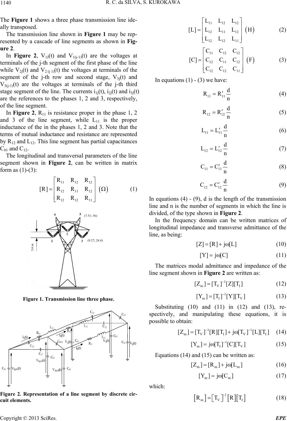 R. C. da SILVA, S. KUROKAWA 1140 The Figure 1 shows a three phase transmission line ide- ally transposed. The transmission line shown in Figure 1 may be rep- resented by a cascade of line segments as shown in Fig- ure 2. In Figure 2, V1J(t) and V1(j-1)(t) are the voltages at terminals of the j-th segment of the first phase of the line while V2j(t) and V2 (j 1)(t) the voltages at terminals of the segment of the j-th row and second stage, V3j(t) and V3(j-1)(t) are the voltages at terminals of the j-th third stage segment of the line. The currents i1j(t), i2j(t) and i3j(t) are the references to the phases 1, 2 and 3, respectively, of the line segment. In Figure 2, R11 is resistance proper in the phase 1, 2 and 3 of the line segment, while L11 is the proper inductance of the in the phases 1, 2 and 3. Note that the terms of mutual inductance and resistance are represented by R12 and L12. This line segment has partial capacitances C01 and C12. The longitudinal and transversal parameters of the line segment shown in Figure 2, can be written in matrix form as (1)-(3): 11 12 12 1211 12 12 12 11 RRR [R]RRR RRR (1) 1 23 45 (9.27; 24.4) (7.51; 36) 3.6 m Figure 1. Transmission line three phase. Figure 2. Representation of a line segment by discrete cir- cuit elements. 11 12 12 1211 12 12 12 11 LLL [L]LLL H LLL (2) 11 12 12 1211 12 12 12 11 CCC [C]CCC F CCC (3) In equations (1) - (3) we have: 11 11 d RR n (4) 12 12 d RR n (5) 11 11 d LL n (6) 12 12 d LL n (7) 11 11 d CC n (8) 12 12 d CC n (9) In equations (4) - (9), d is the length of the transmission line and n is the number of segments in which the line is divided, of the type shown in Figure 2. In the frequency domain can be written matrices of longitudinal impedance and transverse admittance of the line, as being: [Z][R]j [L] (10) [Y]j [C] (11) The matrices modal admittance and impedance of the line segment shown in Figure 2 are written as: 1 mV [Z][T][Z][T ] I I V m (12) 1 mI V [Y][T ][Y][T] (13) Substituting (10) and (11) in (12) and (13), re- spectively, and manipulating these equations, it is possible to obtain: 11 mVI V [Z ][T] [R][T]j[T] [L][T] (14) 1 mI [Y]j[T][C][T] (15) Equations (14) and (15) can be written as: mm [Z ][R]j[L ] (16) m [Y ]j[C] m (17) which: 1 mV RTRT I (18) Copyright © 2013 SciRes. EPE 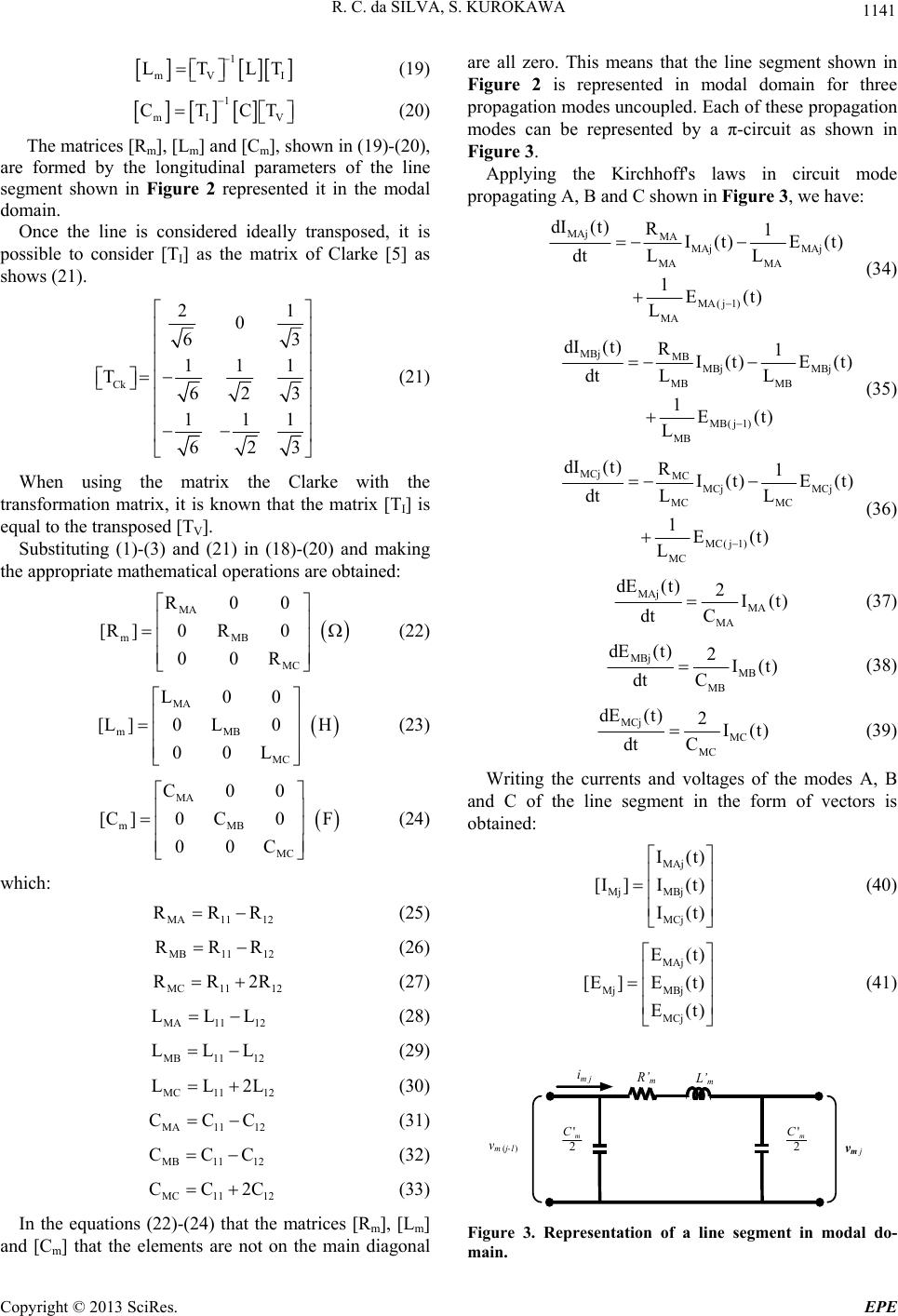 R. C. da SILVA, S. KUROKAWA 1141 1 mV LTLT I (19) 1 mI V CTCT (20) The matrices [Rm], [Lm] and [Cm], shown in (19)-(20), are formed by the longitudinal parameters of the line segment shown in Figure 2 represented it in the modal domain. Once the line is considered ideally transposed, it is possible to consider [TI] as the matrix of Clarke [5] as shows (21). Ck 21 0 63 111 T623 111 623 (21) When using the matrix the Clarke with the transformation matrix, it is known that the matrix [TI] is equal to the transposed [TV]. Substituting (1)-(3) and (21) in (18)-(20) and making the appropriate mathematical operations are obtained: MA mMB MC R00 [R]0R0 00R (22) MA mMB MC L00 [L]0L0 H 00L (23) MA mMB MC C00 [C]0C0 F 00C (24) which: MA11 12 RRR (25) MB1112 RRR (26) MC 1112 RR2R (27) MA11 12 LLL (28) MB1112 LLL (29) MC 1112 LL2L (30) MA11 12 CCC (31) MB11 12 CCC (32) MC 1112 CC2C (33) In the equations (22)-(24) that the matrices [Rm], [Lm] and [Cm] that the elements are not on the main diagonal are all zero. This means that the line segment shown in Figure 2 is represented in modal domain for three propagation modes uncoupled. Each of these propagation modes can be represented by a π-circuit as shown in Figure 3. Applying the Kirchhoff's laws in circuit mode propagating A, B and C shown in Figure 3, we have: MAj MA MAj MAj MA MA MA(j1) MA dI (t)R1 I(t) E(t) dt LL 1 E(t) L (34) MBj MB MBj MBj MB MB MB( j1) MB dI (t)R1 I(t) E(t) dt LL 1 E(t) L (35) MCj MC MCj MCj MC MC MC( j1) MC dI (t)R1 I (t)E (t) dt LL 1 E(t) L (36) MAj MA MA dE (t)2I(t) dt C (37) MBj MB MB dE (t)2I(t) dt C (38) MCj MC MC dE (t)2I(t) dt C (39) Writing the currents and voltages of the modes A, B and C of the line segment in the form of vectors is obtained: MAj Mj MBj MCj I(t) [I ]I(t) I(t) (40) MAj Mj MBj MCj E(t) [E ]E(t) E(t) (41) i m j ' 2 m C ' 2 m C L’ m R’ m v m j v m (j-1 ) Figure 3. Representation of a line segment in modal do- main. Copyright © 2013 SciRes. EPE 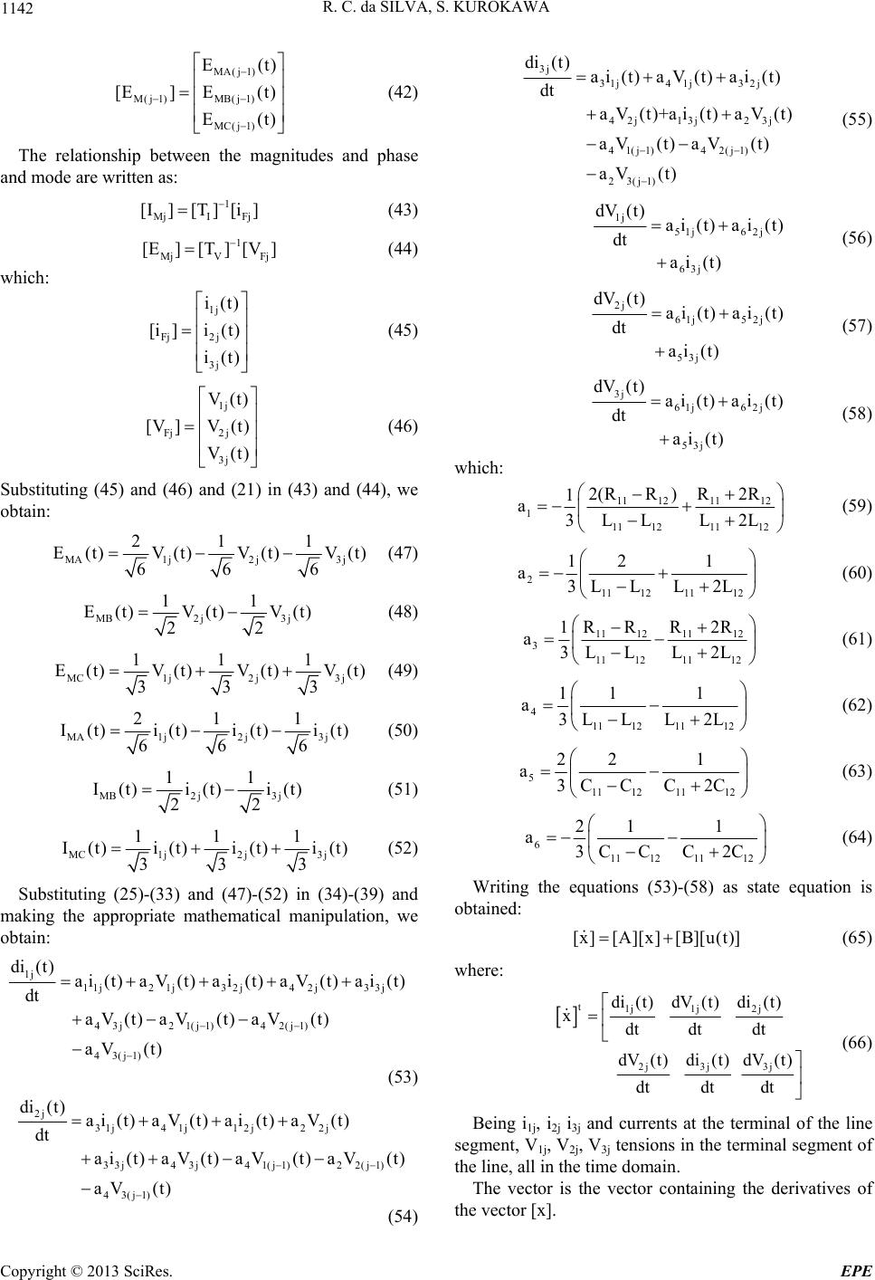 R. C. da SILVA, S. KUROKAWA 1142 MA( j1) M(j1)MB(j1) MC( j1) E(t [E] E(t) E(t ) ) (42) The relationship between the magnitudes and phase and mode are written as: 1 MjI Fj [I][T ][i] (43) 1 MjV Fj [E][T ][V ] (44) which: 1j Fj2 j 3j i(t) [i ]i(t) i(t) (45) 1j Fj2 j 3j V(t) [V ]V(t) V(t) (46) Substituting (45) and (46) and (21) in (43) and (44), we obtain: MA1j2 j3j 21 1 E(t)V(t) V(t) V(t) 66 6 (47) MB2 j3 j 11 E(t)V (t)V (t) 22 (48) MC1j2 j3 j 111 E(t)V(t) V(t) V(t) 333 (49) MA1j2 j3j 21 1 I(t)i(t)i(t)i(t) 666 (50) MB2 j3 j 11 I(t)i (t)i (t) 22 (51) MC1j2 j3 j 111 I(t)i(t) i(t) i(t) 333 (52) Substituting (25)-(33) and (47)-(52) in (34)-(39) and making the appropriate mathematical manipulation, we obtain: 1j 11j21j32j42j33j 43j 21(j1) 42(j1) 43(j1) di (t)ai(t)aV(t) ai(t) aV(t) ai(t) dt aV(t)aV(t)aV(t) aV(t) (53) 2j 31j4 1j12j2 2j 3 3j43j41(j 1)22(j 1) 43(j1) di (t)ai(t) aV(t) ai(t)aV(t) dt ai(t)aV(t)aV(t)aV(t) aV(t) 3j 31j41j3 2j 42j 13j23j 41(j 1)42(j 1) 23(j1) di (t)ai(t)aV(t)ai(t) dt aV(t)+ai(t)aV(t) aV(t)aV(t) aV(t) (55) 1j 51j6 2j 63j dV (t)ai(t)ai(t) dt ai(t) (56) 2j 61j52j 53j dV (t)ai(t)ai(t) dt ai(t) (57) 3j 61j 62j 53j dV (t)ai (t)ai(t) dt ai(t) (58) which: 11 121112 1 11 121112 2(RR )R2R 1 a3LL L2L (59) 2 11 121112 12 1 a3L LL 2L (60) 11 121112 3 11 121112 RR R2R 1 a3L LL2L (61) 4 11 121112 111 a3L LL 2L (62) 5 11 121112 22 1 a3C CC2C (63) 6 11 121112 21 1 a3C CC2C (64) Writing the equations (53)-(58) as state equation is obtained: [x][A][x] [B][u(t)] (65) where: t1j1j 2j 2j 3j3j di(t)dV (t)di(t) x dt dtdt dV(t)di(t)dV (t) dtdt dt (66) (54) Being i1j, i2j i3j and currents at the terminal of the line segment, V1j, V2j, V3j tensions in the terminal segment of the line, all in the time domain. The vector is the vector containing the derivatives of the vector [x]. Copyright © 2013 SciRes. EPE 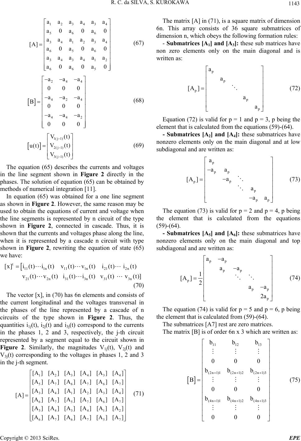 R. C. da SILVA, S. KUROKAWA 1143 123434 566 341234 656 343412 665 aaaaaa a0a0a0 aaaaaa [A] a0a0a0 aa aaaa a0a0a0 (67) 244 424 442 aaa 000 aaa B000 aaa 000 (68) 1( j1) 2( j1) 3( j1) V(t) V(t) u(t) V(t) (69) The equation (65) describes the currents and voltages in the line segment shown in Figure 2 directly in the phases. The solution of equation (65) can be obtained by methods of numerical integration [11]. In equation (65) was obtained for a one line segment as shown in Figure 2. However, the same reason may be used to obtain the equations of current and voltage when the line segments is represented by n circuit of the type shown in Figure 2, connected in cascade. Thus, it is shown that the currents and voltages phase along the line, when it is represented by a cascade n circuit with type shown in Figure 2, rewriting the equation of state (65) we have: t 111n 11 1n212n 212n313n313n [x]i(t)i(t) v(t)v(t) i(t) i(t) v(t)v(t) i(t)i(t) v(t) v(t)] (70) The vector [x], in (70) has 6n elements and consists of the current longitudinal and the voltages transversal in the phases of the line represented by a cascade of n circuits of the type shown in Figure 2. Thus, the quantities i1j(t), i2j(t) and i3j(t) correspond to the currents in the phases 1, 2 and 3, respectively, the j-th circuit represented by a segment equal to the circuit shown in Figure 2. Similarly, the magnitudes V1j(t), V2j(t) and V3j(t) corresponding to the voltages in phases 1, 2 and 3 in the j-th segment. 123434 576767 341234 675767 343412 676757 [A][A][A] [A][A] [A] [A][A ][A ][A ][A ][A ] [A ][A][A][A][A ][A] [A] [A][A ][A][A ][A ][A ] [A] [A][A] [A] [A] [A] [A ][A ][A ][A ][A ][A ] (71) The matrix [A] in (71), is a square matrix of dimension 6n. This array consists of 36 square submatrices of dimension n, which obeys the following formation rules: - Submatrices [A1] and [A3]: these sub matrices have non zero elements only on the main diagonal and is written as: p p p p p a a [A ] a a (72) Equation (72) is valid for p = 1 and p = 3, p being the element that is calculated from the equations (59)-(64). - Submatrices [A2] and [A4]: these submatrices have nonzero elements only on the main diagonal and at low subdiagonal and are written as: p pp p p p p p a aa a [A ] a aa (73) The equation (73) is valid for p = 2 and p = 4, p being the element that is calculated from the equations (59)-(64). - Submatrices [A5] and [A6]: these submatrices have nonzero elements only on the main diagonal and top subdiagonal and are written as: pp pp p p p p aa aa 1 [A ]2aa 2a (74) The equation (74) is valid for p = 5 and p = 6, p being the element that is calculated from (59)-(64). The submatrices [A7] rest are zero matrices. The matrix [B] is of order 6n x 3 which are written as: 11 1213 (2n 1)1(2n 1)2(2n 1)3 (4n 1)1(4n 1)2(4n 1)3 bbb 000 bb b B 000 bb b 000 (75) Copyright © 2013 SciRes. EPE 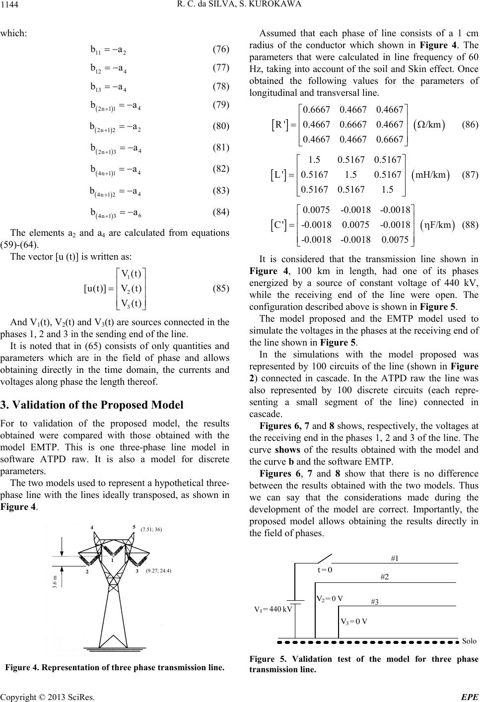 R. C. da SILVA, S. KUROKAWA 1144 which: 11 2 b a (76) 12 4 b a (77) 13 4 b a (78) 4 2n11 b a (79) 2 2n1 2 b a (80) 4 2n13 b a (81) 4 4n11 b a (82) 4 4n1 2 b a (83) 6 4n13 b a (84) The elements a2 and a4 are calculated from equations (59)-(64). The vector [u (t)] is written as: 1 2 3 V(t) [u(t)]V(t) V(t) (85) And V1(t), V2(t) and V3(t) are sources connected in the phases 1, 2 and 3 in the sending end of the line. It is noted that in (65) consists of only quantities and parameters which are in the field of phase and allows obtaining directly in the time domain, the currents and voltages along phase the length thereof. 3. Validation of the Proposed Model For to validation of the proposed model, the results obtained were compared with those obtained with the model EMTP. This is one three-phase line model in software ATPD raw. It is also a model for discrete parameters. The two models used to represent a hypothetical three- phase line with the lines ideally transposed, as shown in Figure 4. 1 23 45 (9.27; 24.4) (7.51; 36) 3.6 m Figure 4. Representation of three phase transmission line. Assumed that each phase of line consists of a 1 cm radius of the conductor which shown in Figure 4. The parameters that were calculated in line frequency of 60 Hz, taking into account of the soil and Skin effect. Once obtained the following values for the parameters of longitudinal and transversal line. 0.6667 0.46670.4667 R'0.46670.66670.4667 /km 0.4667 0.46670.6667 (86) 1.50.5167 0.5167 L'0.51671.50.5167 mH/km 0.5167 0.51671.5 (87) 0.0075-0.0018-0.0018 C'-0.00180.0075-0.0018 F/km -0.0018 -0.00180.0075 (88) It is considered that the transmission line shown in Figure 4, 100 km in length, had one of its phases energized by a source of constant voltage of 440 kV, while the receiving end of the line were open. The configuration described above is shown in Figure 5. The model proposed and the EMTP model used to simulate the voltages in the phases at the receiving end of the line shown in Figure 5. In the simulations with the model proposed was represented by 100 circuits of the line (shown in Figure 2) connected in cascade. In the ATPD raw the line was also represented by 100 discrete circuits (each repre- senting a small segment of the line) connected in cascade. Figures 6, 7 and 8 shows, respectively, the voltages at the receiving end in the phases 1, 2 and 3 of the line. The curve shows of the results obtained with the model and the curve b and the software EMTP. Figures 6, 7 and 8 show that there is no difference between the results obtained with the two models. Thus we can say that the considerations made during the development of the model are correct. Importantly, the proposed model allows obtaining the results directly in the field of phases. Figure 5. Validation test of the model for three phase transmission line. Copyright © 2013 SciRes. EPE 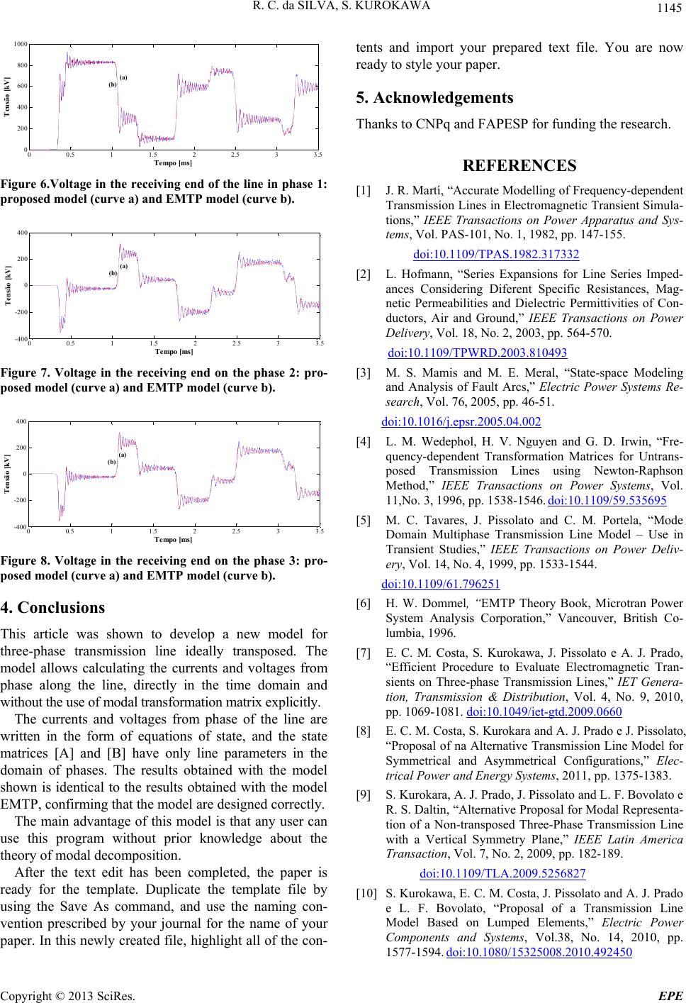 R. C. da SILVA, S. KUROKAWA 1145 00.5 11.5 22.5 33.5 0 200 400 600 800 1000 Tempo [ms] Tensão [kV] (a) (b) Figure 6.Voltage in the receiving end of the line in phase 1: proposed model (curve a) and EMTP model (curve b). 00.5 11.522.533.5 -400 -200 0 200 400 Tempo [ms] Tensão [kV] (a) (b) Figure 7. Voltage in the receiving end on the phase 2: pro- posed model (curve a) and EMTP mode l (c urve b). 00.5 11.5 22.5 33.5 -400 -200 0 200 400 Tempo [ms] Tensão [kV] (a) (b) Figure 8. Voltage in the receiving end on the phase 3: pro- posed model (curve a) and EMTP mode l (c urve b). 4. Conclusions This article was shown to develop a new model for three-phase transmission line ideally transposed. The model allows calculating the currents and voltages from phase along the line, directly in the time domain and without the use of modal transformation matrix explicitly. The currents and voltages from phase of the line are written in the form of equations of state, and the state matrices [A] and [B] have only line parameters in the domain of phases. The results obtained with the model shown is identical to the results obtained with the model EMTP, confirming that the model are designed correctly. The main advantage of this model is that any user can use this program without prior knowledge about the theory of modal decomposition. After the text edit has been completed, the paper is ready for the template. Duplicate the template file by using the Save As command, and use the naming con- vention prescribed by your journal for the name of your paper. In this newly created file, highlight all of the con- tents and import your prepared text file. You are now ready to style your paper. 5. Acknowledgements Thanks to CNPq and FAPESP for funding the research. REFERENCES [1] J. R. Martí, “Accurate Modelling of Frequency-dependent Transmission Lines in Electromagnetic Transient Simula- tions,” IEEE Transactions on Power Apparatus and Sys- tems, Vol. PAS-101, No. 1, 1982, pp. 147-155. doi:10.1109/TPAS.1982.317332 [2] L. Hofmann, “Series Expansions for Line Series Imped- ances Considering Diferent Specific Resistances, Mag- netic Permeabilities and Dielectric Permittivities of Con- ductors, Air and Ground,” IEEE Transactions on Power Delivery, Vol. 18, No. 2, 2003, pp. 564-570. doi:10.1109/TPWRD.2003.810493 [3] M. S. Mamis and M. E. Meral, “State-space Modeling and Analysis of Fault Arcs,” Electric Power Systems Re- search, Vol. 76, 2005, pp. 46-51. doi:10.1016/j.epsr.2005.04.002 [4] L. M. Wedephol, H. V. Nguyen and G. D. Irwin, “Fre- quency-dependent Transformation Matrices for Untrans- posed Transmission Lines using Newton-Raphson Method,” IEEE Transactions on Power Systems, Vol. 11,No. 3, 1996, pp. 1538-1546. doi:10.1109/59.535695 [5] M. C. Tavares, J. Pissolato and C. M. Portela, “Mode Domain Multiphase Transmission Line Model – Use in Transient Studies,” IEEE Transactions on Power Deliv- ery, Vol. 14, No. 4, 1999, pp. 1533-1544. doi:10.1109/61.796251 [6] H. W. Dommel, “EMTP Theory Book, Microtran Power System Analysis Corporation,” Vancouver, British Co- lumbia, 1996. [7] E. C. M. Costa, S. Kurokawa, J. Pissolato e A. J. Prado, “Efficient Procedure to Evaluate Electromagnetic Tran- sients on Three-phase Transmission Lines,” IET Genera- tion, Transmission & Distribution, Vol. 4, No. 9, 2010, pp. 1069-1081. doi:10.1049/iet-gtd.2009.0660 [8] E. C. M. Costa, S. Kurokara and A. J. Prado e J. Pissolato, “Proposal of na Alternative Transmission Line Model for Symmetrical and Asymmetrical Configurations,” Elec- trical Power and Energy Systems, 2011, pp. 1375-1383. [9] S. Kurokara, A. J. Prado, J. Pissolato and L. F. Bovolato e R. S. Daltin, “Alternative Proposal for Modal Representa- tion of a Non-transposed Three-Phase Transmission Line with a Vertical Symmetry Plane,” IEEE Latin America Transaction, Vol. 7, No. 2, 2009, pp. 182-189. doi:10.1109/TLA.2009.5256827 [10] S. Kurokawa, E. C. M. Costa, J. Pissolato and A. J. Prado e L. F. Bovolato, “Proposal of a Transmission Line Model Based on Lumped Elements,” Electric Power Components and Systems, Vol.38, No. 14, 2010, pp. 1577-1594. doi:10.1080/15325008.2010.492450 Copyright © 2013 SciRes. EPE |