Accuracy Improvement in CCT Estimation of Power Systems by iRprop-RAN Hybrid Neural Network

doi:10.4236/epe.2013.54B191

Paper Menu >>

Journal Menu >>

Energy and Power Engineering, 2013, 5, 999-1004

doi:10.4236/epe.2013.54B191 Published Online July 2013 (http://www.scirp.org/journal/epe)

Accuracy Improvement in CCT Estimation of Power

Systems by iRprop-RAN Hybrid Neural Network

Teruhisa Kumano, Shinjiro Netsu

Department of Electronics and Bioinformatics, Meiji University, Kawasaki, Japan

Email: [email protected]

Received March, 2013

ABSTRACT

This paper proposes a new Initial CCT (Critical Clearing Time) estimation method using a hybrid neural network com-

posed of iRprop (Improving the Resilient back PROPation Algorithm) and RAN (Resource Allocation Network). In

transient stability study, CCT evaluation is very important bu t time consuming due to the fact it needs many iteration of

time domain simulations gradu ally increasing the fault clearing time. The key to reduce th e required computing time in

this process is to find accurate initial estimation of CCT by a certain handy method before going to the iterative stage.

As one of the strongest candidates of this handy method is the utilization of the pattern recognition ability of neural

networks, which enable us to jump to a close estimation of the real CCT without any heavy computing burden. This

paper proposes a new hybrid neural network which is a combination of the well-known iRprop and RAN. In the pro-

posed method, the outputs of the hidden units of RAN are modified by multiplying the contribution factors calculated

by an additional iRprop network. Numerical studies are done using two different test systems for the purpose of con-

firming the validity of the proposal. The result of the proposed method is the best. Properly evaluating the contribution

of each input to the hidden units, the estimation error obtained by the proposed method is improved further than the

original RAN based estimation.

Keywords: Critical Clearing Time; Estimation; Power System; iRprop; Resource Allocation Network

1. Introduction

In large power systems operation, stability check in the

contingency analysis is always important. In particular,

in these two years, we, Japanese electric power engineers,

cannot depend upon the strong power supply from the

nuclear power plants and the basic power flow pattern is

different from the original schedule. It implies that every

daily grid operation needs more careful study, in which

stability check should be done. The long and narrow

power corridor is, in a sense, inevitable due to the geo-

graphical restriction of our country, which makes the

stability the main restricting factor for the long and heavy

power transmission.

One of the biggest problems in the transient stability

constrained contingency analysis is the long computing

time required. Transient stability study itself is a typical

time consuming calculation. Here, we need to iterate

dynamic simulation many times gradually increasing

power flow or fault clearing time to reach their critical

value. Comparing these two, the critical clearing time

(CCT) is easy to calculate and is often used. For the fast

evaluation of CCT, we need accurate initial guess of the

clearing time. If we can start from close guess, the re-

quired time to get the true CCT can be shorter. Since the

power flow pattern in the whole system gives a substan-

tial effects on the resultant CCT, it can be expected that

we can accurately estimate CCT if the important vari-

ables such as the specified values of the active and reac-

tive power at each node is given.

Many methods based on so called artificial neural

network (ANN) techniques have been studied for this

initial guess. Ikenono et al proposed to use BP (back

propagation) based ANN [1]. Bettiol et al proposed to

use RBF (Radial Basis Function) network for this pur-

pose [2]. The authors ourselves studied this problem and

proposed to use support vector machine [3] and rele-

vance vector machine [4]. Once properly trained, ANN

can recognize the given input pattern and make classifi-

cation or give a regression in a short computing time.

Because of its nonlinear knowledge representation ability,

it has been a strong candidate for this initial estimator.

However, even after the above mentioned research ef-

forts, it still remains as a research theme and not a real

field application.

In this paper, a new ANN method is proposed for the

above stated purpose. In this proposal so called RAN

(Resource Allocation Network) is coupled with iRprop

(Improving the Rprop Learning Algorithm, in which

T. KUMANO, S. NETSU

1000

Rprop stands for Resilient backPROPagation). RAN is

one type of RBF network, but it has a strong adap tability

given by the hidden layer adjustment. RAN and its modi-

fications are applied to various fields and makes a con-

siderable contribution. [5-7] The details of iRprop and

RAN will be described in the next chapter.

This paper is constructed as follows. Chapter 2 ex-

plains the proposal in this paper together with the basics

related to iRprop and RAN. Chapter 3 describes our tran-

sient stability problem, followed by numerical examples

written in Chapter 4. In Chapter 5 concluding remarks

are stated.

2. Related Networks and the Proposal

2.1. iRprop

The proposed method in this paper is a hybrid of iRprop

and RAN. The former (more strictly, iRprop+) is an im-

proved version of BP (Back Propagation) ANN. While

BP shifts the weight of each connection by the gradient

and needs the partial derivative calculated, iRprop only

watches the sign of the partial derivative. Its light com-

puting cost enables us to apply this method to many

fields.

The mathematical description of its learning algorithm

is as follows [8]. The weight of each connection is wij and

it is shifted by the following algorithm depending upon

the sign of(t-1)( )







, where E stands for the sum of

the output error. In the following equations, coefficient



+ and



- should satisfy 0<



-<1<



+. max and min imply

the upper and lower limits of ij(t)

i) In case (t-1)( )









()( 1)max

()

() ()

(1) ()()

min ,

ij ij

ttt

ijij ij

wsign

www







  





 









ii) in case (t-1)( )









()( 1)min

()(1)(1) ()(1)

(1) ()

()

max ,

if then

otherwise

ij ij

tttt t

ijijij

ij ij

EEwww









  













iii) in case (t-1)( )







()

() ()

(1) ()()

ij ij

ttt

ijij ij

wsign

www









 









2.2. RAN

On the other hand, RAN is composed of 1) a network, 2)

strategy for allocating new units, and 3) a learning rule

for refining the n etwork. [9] It is based on the concept of

RBF (Radial Basis Function) machine. [2] Let I be the

input. Using c and



2, the center and the variance of the

RBF, y, the output of the hidden unit, is computed by

exp(/).

ipj

yIc



 (1)

where j, i, and p stand for the suffix fo r th e number of th e

hidden units, those of the input units, and sample id re-

spectively. The network output z is calculated, using the

weight h and the output bias



, as follows.

kki

zhy









(2)

RAN also learns so as to minimize the sum of the

squared output error E. When the newly obtained input is

not found in the experience so far (far from the used data

sample obtained in the history), another hidden unit is

added. This algorithm is formulated as follows.

if E>



and ||x-cnearest||>



then

j=j+1

cji=xpi



j2=k || x-cnearest||

hji=Tpk-zk

where Tpk is the teacher signal.

2.3. The Proposed Method

RAN modifies its structure by adding a new hidden unit

only in the case where the output error and the difference

between the input data and the nearest center of the ex-

isting radial basis functions are big enough simultane-

ously. However, in our specific problem, the input data

contain various quantity such as vo ltag e, power, and fault

location etc.. Some input might have strong effects on the

inputs to the hidden layer, but others not. In the proposed

method, this difference in the degree of the effects on the

hidden layer is assessed by an additional iRprop network

which connects every input variable with every hidden

unit.

Learning is done simultaneously in this additional iR-

prop network and the obtained weight of each connection

is multiplied to the difference between each input and the

nearest center, the sum of which is used to calculate the

output of the hidden units. Using y, I, c, and



of the

same meaning as in the previous section, the output of

T. KUMANO, S. NETSU 1001

the hidden unit y is written as

exp( )

pj i

cef





 (3)

where th e new coeff icien t ef implies the degree of effects

and is calculated by the f ol l owing for mula;

ef wj

which is the sum of the weights in th e above stated addi-

tional iRprop network. The proposed network takes the

form shown in Figure 1. The additional part on the top

(boxed in the broken rectangle) is iRprop, the sum of the

connection weight of which is ef and is multiplied to the

distance between input Ik and the nearest center as shown

in Equation (3). Figure 2 shows the type of input/output

data used in the proposed method.

3. Studied Problem

3.1. Data Preparation Procedure

In our particular problem, so called CCT (Critical Clear-

ing Time) is the target of the estimation. CCT is the

Figure 1. The structure of the proposed network.

gen output load power LFdata & transmission loss gen volt. fault location

CCT (Critic al C learing Time)

Figure 2. Inputs and output of the pr oposed network.

maximum fault duration which do es not cause instab ility.

In order to obtain the teacher signal fed to the proposed

method, the true CCT, dynamic simulation is run many

times. It is true that this is only a result of simulation

analysis, but is treated as the correct CCT.

Using CPAT (CRIEPI’s Power system Analysis Tool)

[10], a de facto standard stability analysis program in

many Japanese power utilities, the power system tran-

sient behavior is computed under various conditio ns such

as initial load flow, fault location etc., where the fault

clearing time is gradually increased. The assumed long-

est clearing time which causes no transient stability

problem such as out of step within the predetermined

time range (described later in Tables 1 and 2) is consid-

ered as CCT.

Table 1. Simulation Condition in 9 Node System.

item setting

gen. output increased at the constant rate to keep up with

the total demand

load demand 80, 90, 100, 110, 120%

input data gen and load power, branch power flow, nodal

voltage, branch loss, fault location

output CCT

fault locations sending end of all branches

fault type 3LG (three lines g r o u n d ed)

criterion of SOinternal bus angle > 180 deg

etc simulation quits after t=0.5sec

Table 2. Simulation Condition in 47 Node System.

item setting

gen. output

output from a gen in Area A is increased by

0.1pu step while the output from all gens in

Area B are reduced at the same rate to keep the

total demand unchan g ed

load demand 100% unchanged

input data gen power, branch power flow, nodal voltage,

fault location

output CCT

fault locations at HV bus of the step-up transformer of gen-

erators 8,9,10

fault type 3LG (three lines gr o un d ed)

criterion of SOinternal bus angle > 180 deg

etc simulation quits after t=4.0sec

3.2. Study Power Systems

Two model systems shown in Figures 3 and 4 are stud-

ied. The details such as machine constants used in the 9

bus model can be found in [11]. In the study of the 47

T. KUMANO, S. NETSU

1002

4. Numerical Study

node system, base loading is set as its standard, or 100%

loading condition. The analysis condition is summarized

in Tables 1-3. For the purpose of confirmation of the validity of the

proposed method, it is compared with the two existing

networks, BP (the classical Back Propagation based net-

work) and iRprop. The parameters are determined by try

and error. They are summarized in Tables 5-6.

3.3. Transient Stability Analysis

The transient stability an alysis is done, which is required

to get the input and the teacher signal fed to our ANN, as

explained below. The simulation condition used for the

nine bus model is shown in Table 1. On the other hand,

Table 2 shows that used in 47 node model. In Table 2,

two area s are refereed in th e description of th e procedure

how the generator outputs are changed. Area A means

the northern part of the 47 node system, which includes

the three generators G8 - G10. The remaining region is

Area B. Tables 3 and 4 show the generation/demand

settings for each case.

Table 3. Generator Condition in 47 Node System.

gen No gen type voltage capacity

1 LNG 1.01pu 8240MVA

2 nuclear 1.00pu 12940MVA

3 pumped storage1.02pu 7060MVA

4 coal 1.01pu 12940MVA

5 pumped storage1.02pu 7060MVA

6 coal 1.02pu 12940MVA

7 nuclear 1.00pu 12940MVA

8 oil 1.00pu 8240MVA

9 oil 1.00pu 8240MVA

10 oil 1.02pu 5880MVA

G3G2

Figure 3. Anderson and Fouad 9 bus system.

G1 0

G2 G4

G7 G6

G9 G8

(10) (20)(37)(36)

(47) (19)

(9) (8)

(18)

(1)

(11) (12)

(2) (4)

(14)

(3)

(13)

(25)

(44)

(26)

(21)

(22)

(38) (39)

(24)

(23)

(27)

(40) (41)

(45)

(30)

(29)

(28)

(15)

(5)

(7)

(17)

(46)

(31) (32)

(33)

(42) (43)

(34)

(35)

(16)

(6)

<10> <52>

<40> <39>

<9>

<51 >

<37><38>

<50 >

<8>

<36>

<7> <6>

<153><53>

<32><30 ><28><25 ><22> <124><24>

<123><23>

<4><2>

<1>

<11>

<13>

<12>

<14>

<41> <42>

<15><20> <120>

<19><16>

<18> <118>

<117><17>

<43>

<27>

<26> <126>

<48> <49>

<35> <135>

<31> <33>

<34>

<45> <46><44>

<29>

<5>

<47>

<21>

<3>

Figure 4. IEEJ standard 47 bus model system EAST-10.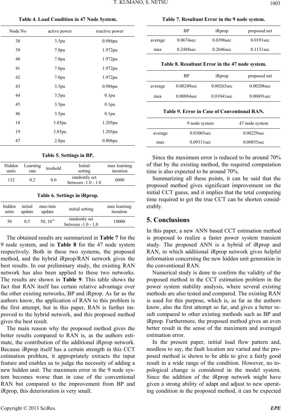

T. KUMANO, S. NETSU 1003

Table 4. Load Condition in 47 Node System.

Node No active power reactive power

38 3.5pu 0.986pu

39 7.0pu 1.972pu

40 7.0pu 1.972pu

41 7.0pu 1.972pu

42 7.0pu 1.972pu

43 3.5pu 0.986pu

44 3.5pu 0.1pu

45 3.5pu 0.1pu

46 3.5pu 0.1pu

18 3.85pu 1.205pu

19 3.85pu 1.205pu

47 2.8pu 0.806pu

Table 5. Settings in BP.

Hidden

units Learning

rate treshold Initial

setting max learning

iteration

132 0.2 0.0 ra ndomly set

between -1.0 - 1.0 6000

Table 6. Settings in iRprop.

hidden

units initial

update max/min

update initial setting max lear n ing

iteration

30 0.5 50, 10-6 randomly set

between -1.0 - 1.0 10000

The obtained results are summarized in Table 7 for the

9 node system, and in Table 8 for the 47 node system

respectively. Both in these two systems, the proposed

method, and the hybrid iRprop/RAN network gives the

best results. In our preliminary study, the existing RAN

network has also been applied to these two networks.

The results are shown in Table 9. This table shows the

fact that RAN itself has certain relative advantage over

the other existing networks, BP and iRprop. As far as the

authors know, the application of RAN to this problem is

the first attempt, but in this paper, RAN is further im-

proved to the hybrid network, and this proposed method

gives the be s t result .

The main reason why the proposed method gives the

better results compared to RAN is, as the authors esti-

mate, the contribution of the additional iRprop network.

Because iRprop itself has a certain strength in this CCT

estimation problem, it appropriately extracts the input

feature and enables us to judge the necessity of adding a

new hidden unit. The maximum error in the 9 node sys-

tem becomes worse than in case of the conventional

RAN but compared to the improvement from BP and

iRprop, this deterioration is very small.

Table 7. Resultant Error in the 9 node system.

BP iRprop proposed net

average0.0674sec 0.0396sec 0.0191sec

max 0.2488sec 0.2646sec 0.1131sec

Table 8. Resultant Error in the 47 node system.

BP iRprop proposed net

average0.00249sec 0.00263sec 0.00208sec

max 0.00884sec 0.01041sec 0.00691sec

Table 9. Error in Case of Conventional RAN.

9 node system 47 node system

average 0.03003sec 0.00229sec

max 0.09311sec 0.00855sec

Since the maximum error is reduced to be around 70%

of that by the existing method, the required computation

time is also expected to be around 70%.

Summarizing all these points, it can be said that the

proposed method gives significant improvement on the

initial CCT guess, and it implies that th e total computing

time required to get the true CCT can be shorten consid-

erably.

5. Conclusions

In this paper, a new ANN based CCT estimation method

is proposed to realize a faster power system transient

study. The proposed ANN is a hybrid of iRprop and

RAN, in which additional iRprop network gives helpful

information concerning the new hidden unit generation in

the conventional RAN.

Numerical study is done to confirm the validity of the

proposed method in the CCT estimation problem in the

power system stability analysis, where several existing

methods are also tested and compared. The existing RAN

is used for this purpose, which is, as far as the authors

know, also the first attempt so far, and gives a better re-

sult compared to other existing methods such as BP and

iRprop. Furthermore, the proposed method gives an even

better result in the sense of the maximum and averaged

estimation error.

In the present paper, initial load flow pattern and,

needless to say, the fault location are varied and the pro-

posed method is shown to be able to give a fairly good

result in a wide range of the condition. However, no to-

pological change is considered in the model system.

Since the addition of the iRprop network might have

given a strong ability of adapt and adjust to new operat-

ing condition in the proposed method, it can be expected

T. KUMANO, S. NETSU

1004

that our method might be well applied in a bigg er condi-

tion change such as topological. Due to the new grid par-

ticipants such as distributed generators, the grid configu-

ration might be more frequently changed from now,

which might affects the power transmission capability of

the trunk system. It implies that the importance of the

proposed method will become bigger and bigger in near

future.

REFERENCES

[1] K. Ikenono and S. Iwamoto, “Generalization of Transient

Stability Solution using Neural Network Theory,” Trans

IEEJ, Vol. 111, No. 7, 1991, pp. 723-728.

[2] A. L. Bettiol, A. Souza, J. L. Todesco and J. R. Tesch, Jr,

“Estimation of Critical Clearing Times Using Neural

Networks,” 2003 IEEE Bologna Power Tech Conference

Proceedings. doi:10.1109/PTC.2003.1304446

[3] H. Takahashi and T. Kumano, “Available Transfer Capa-

bility Screening Considering Transient Stability by Sup-

port Vector Machine,” 2008 IEEE PES General Meeting,

Pittsburgh. doi:10.1109/PES.2008.4596499v

[4] A. Wada and T. Kumano, “Fast Estimation of Transient

Stability Cconstrained ATC by Relevance Vector Ma-

chine,” IEEE 2nd International Power and Energy Con-

ference, 2008, doi:10.1109/PECON.2008.4762451v

[5] B. S. Mahanand, S. Suresh, N. Sundararajan, M. A. Ku-

mar, “Alzheimer's Disease Detection Using a

Self-adaptive Resource Allocation Network classifier,”

The 2011 International Conference on Neural Networks,

pp. 1930-1934.doi:10.1109/IJCNN.2011.6033460

[6] S. Shanthi and V. M. A. Bhaskaran, “Computer Aided

Detection and Classification of Mammogram Using

Self-adaptive Resource Allocation Network Classifier,”

2012 International Conference on Pattern Recognition,

Informatics and Medical Engineering (PRIME), pp.

284-289. doi:10.1109/ICPRIME.2012.6208359

[7] H. C. Lou and W. Z. Dai, “A Novel Non-linear Model

Predictive Controller Based on Minimal Resource Allo-

cation Network and Its Application in CSTR PH Proc-

ess,” 7th World Congress on Intelligent Control and

Automation, 2008. WCICA 2008, pp. 5672-5676.

doi:10.1109/WCICA.2008.4593855v

[8] C. Igel and M. Husken, “Empirical Evaluation of the

Improved Rprop Learning Algorithms,” Neurocomput-

ing, Vol. 50, 2003, pp. 105-123.

doi:10.1016/S0925-2312(01)00700-7

[9] J. Platt, “A Resource-Allocating Network for Function

Interpolation,” Neural Computation, Vol. 3, No. 2, 1991,

pp. 213-225.doi:10.1162/neco.1991.3.2.213v

[10] Y. Kitauchi, “Scheme of Power System Stability En-

hancement using Margin to Apparatus Limitation (Part II)

－Verification of Power System Stability Improvement

using Highly Voltage Control on IEEJ WEST 30-machine

System Model－”, CRIEPI REPORT R04010, 2005.

[11] P. M. Anderson and A. A. Fouad, Power System Control

and Stability, Iowa State University Press, 1977.