Adaptive Piecewise Linear Controller for Servo Mechanical Control Systems

doi:10.4236/jamp.2013.15013

Paper Menu >>

Journal Menu >>

Journal of Applied Mathematics and Physics, 2013, 1, 85-92

Published Online November 2013 (http://www.scirp.org/journal/jamp)

http://dx.doi.org/10.4236/jamp.2013.15013

Open Access JAMP

Adaptive P iecewise Linear Controller for Servo

Mechanical Control Systems

Tain-Sou Tsay

Department of Aeronautical Engineering, National Formosa University, Yunlin, Taiwan

Email: [email protected]

Received September 18, 2013; revised October 18, 2013; accepted October 27, 2013

permits unrestricted use, distribution, and reproduction in any medium, provided the original work is properly cited.

ABSTRACT

In this paper, an adaptive piecewise linear control scheme is proposed for improving the performance and response time

of servo mechanical control systems. It is a gain stabilized control technique. No large phase lead compensations or

pole zero cancellations are needed for performance improvement. Large gain is used for large tracking error to get fast

response. Small gain is used between large and small tracking error for good performance. Large gain is used again for

small tracking error to cope with disturbance. It gives an almost command independent response. It can speed up the

rise time while keeping robustness unchanged. The proposed control scheme is applied to a servo system with large

time lag and a complicated electro-hydraulic velocity/position servo system. Time responses show that the proposed

method gives significant improvements for response time and performance.

Keywords: Piecewise Linear Controller; Nonlinear Controller; Adaptive Gain; Servo System

1. Introduction

This template Gain and phase stabilized are two conven-

tional design methods for feedback control systems.

They can be analyzed and designed in gain-phase plots to

get wanted gain margin (GM) and phase margin (PM) or

gain crossover frequency



selected for switching. An adaptive switching algorithm

is used. There is no discontinuous connection between

two systems. Therefore, there is no chattering problem.

Gain scheduling has been used successfully to control

nonlinear systems for many decades and in many differ-

ent applications, such as autopilots and chemical proc-

esses [8-10]. It consisted of many linear controllers for

operating points to cope with large parameter variations.

This concept will be expanded for response time and

performance. Operating points are replaced by fast re-

sponse and good performance conditions and interpola-

tion for gain evaluation is replaced by an adaptive

switching point. It is determined by the filtered command

tracking errors. Nonlinear controllers syntheses using

inverse describing function for use with hard nonlinear

system have been developed for several researchers

[11-14]. They are complicated but effective for nonlinear

systems. In this paper, a simple three segments piecewise

linear controller is proposed. It is easy to analyse and

design. Furthermore, it gives an almost reference input

independent response.





and phase crossover

frequency







[1,2]. The gain crossover frequency is

closely related to the system bandwidth (or rise time).

The phase margin is closely related to performance (or

peak overshoot). In general, fast response time and good

performance can not be obtained simultaneously for

some feedback control systems. For example, the altitude

control system of the airframe with altitude and altitude

rate feedbacks needs large altitude loop gain for fast re-

sponse time and low altitude loop gain for good robust-

ness. It is in conflict with another. A simple and effective

way to solve this problem and better results for those of

linear controllers is generally expected. This is the mo-

tivation of this paper. Variable structure control is a

switching control method for feedback control systems

[3-7]. It gives good performance and robustness for cop-

ing with system uncertainty. But it suffered from chat-

tering problem and state measurements. In this paper, a

fast response system and a good performance system are

The proposed control scheme is applied to a servo

system with large transportation lag and a complicated

electro-hydraulic velocity/position servo system. Time

responses show that the proposed method gives signifi-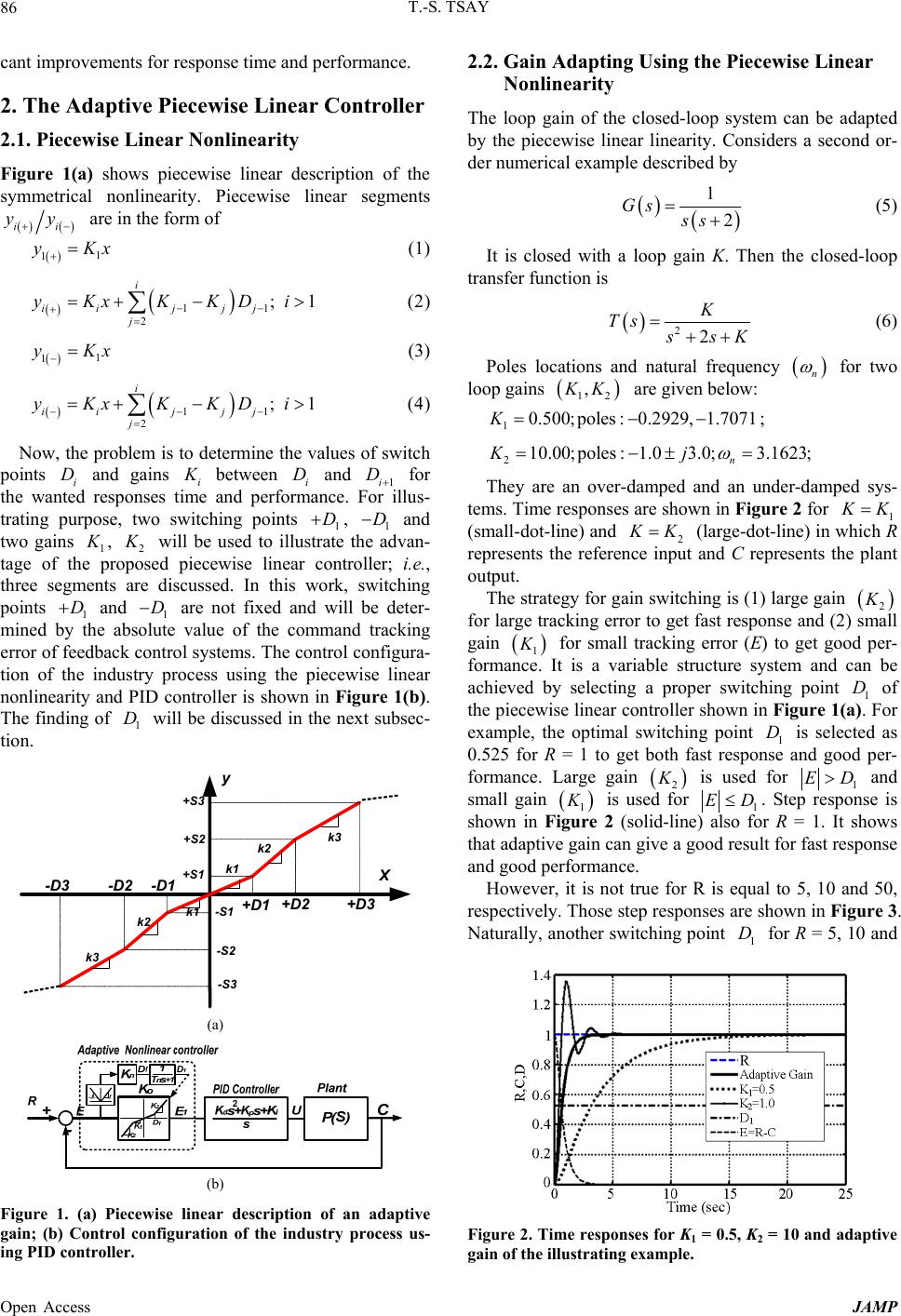

T.-S. TSAY

cant improvements for response time and performance.

2. The Adaptive Piecewise Linear Controller

2.1. Piecewise Linear Nonlinearity

Figure 1(a) shows piecewise linear description of the

symmetrical nonlinearity. Piecewise linear segments

 



are in the form of



x

(1)



;

ii jjj

yKx KKDi







 

 (2)



 (3)



;

ii jjj

yKx KKDi







 

 (4)

Now, the problem is to determine the values of switch

points i and gains i

between i and 1i

D D



for

the wanted responses time and performance. For illus-

trating purpose, two switching points 1, 1

DD



and

two gains 1

, 2

will be used to illustrate the advan-

tage of the proposed piecewise linear controller; i.e.,

three segments are discussed. In this work, switching

points 1 and 1 are not fixed and will be deter-

mined by the absolute value of the command tracking

error of feedback control systems. The control configura-

tion of the industry process using the piecewise linear

nonlinearity and PID controller is shown in Figure 1(b).

The finding of will be discussed in the next subsec-

tion.

DD

+D1

-D1 +D2

-D2 +S1

-S1

+S2

-S2

+S3

-S3

-D3 +D3

(a)

(b)

Figure 1. (a) Piecewise linear description of an adaptive

gain; (b) Control configuration of the industry process us-

ing PID controller.

2.2. Gain Adapting Using the Piecewise Linear

Nonlinearity

The loop gain of the closed-loop system can be adapted

by the piecewise linear linearity. Considers a second or-

der numerical example described by

 

Gs ss

 (5)

It is closed with a loop gain K. Then the closed-loop

transfer function is



 (6)

Poles locations and natural frequency





for two

loop gains





K are given below:

10.500;poles :0.2929,1.7071K



;

210.00;poles:1.03.0;3.1623;







They are an over-damped and an under-damped sys-

tems. Time responses are shown in Figure 2 for 1



(small-dot-line) and 2



(large-dot-line) in which R

represents the reference input and C represents the plant

output.

The strategy for gain switching is (1) large gain





for large tracking error to get fast response and (2) small

gain





for small tracking error (E) to get good per-

formance. It is a variable structure system and can be

achieved by selecting a proper switching point 1 of

the piecewise linear controller shown in Figure 1(a). For

example, the optimal switching point 1 is selected as

0.525 for R = 1 to get both fast response and good per-

formance. Large gain





is used for 1

DE and

small gain





is used for 1

ED. Step response is

shown in Figure 2 (solid-line) also for R = 1. It shows

that adaptive gain can give a good result for fast response

and good performance.

However, it is not true for R is equal to 5, 10 and 50,

respectively. Those step responses are shown in Figure 3.

Naturally, another switching point for R = 5, 10 and

Figure 2. Time responses for K1 = 0.5, K2 = 10 and adaptive

gain of the illustrating example.

Open Access JAMP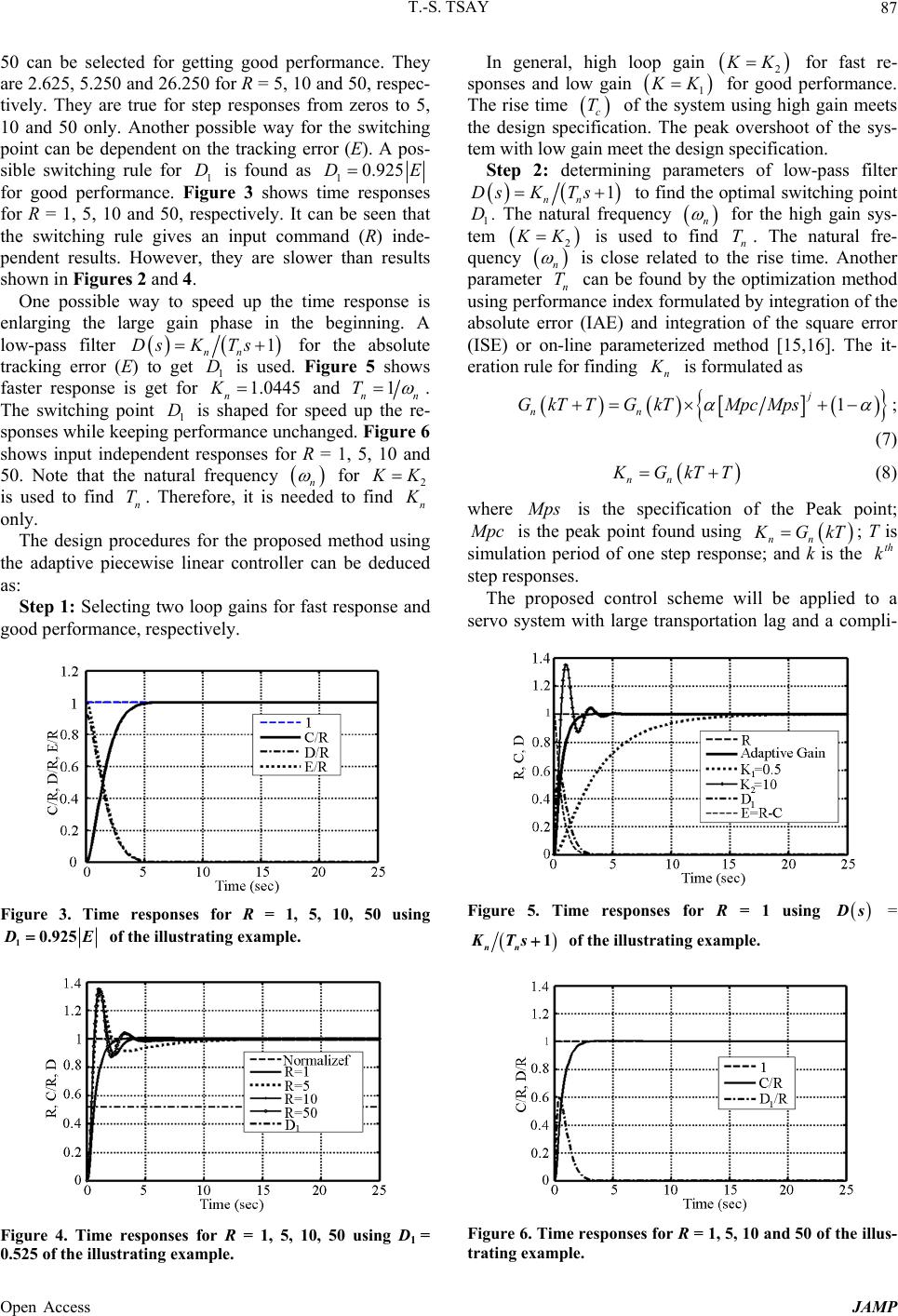

T.-S. TSAY 87

50 can be selected for getting good performance. They

are 2.625, 5.250 and 26.250 for R = 5, 10 and 50, respec-

tively. They are true for step responses from zeros to 5,

10 and 50 only. Another possible way for the switching

point can be dependent on the tracking error (E). A pos-

sible switching rule for 1 is found as D10.925DE

for good performance. Figure 3 shows time responses

for R = 1, 5, 10 and 50, respectively. It can be seen that

the switching rule gives an input command (R) inde-

pendent results. However, they are slower than results

shown in Figures 2 and 4.

One possible way to speed up the time response is

enlarging the large gain phase in the beginning. A

low-pass filter







DsK Ts for the absolute

tracking error (E) to get is used. Figure 5 shows

faster response is get for

K1.0445



and 1





The switching point 1 is shaped for speed up the re-

sponses while keeping performance unchanged. Figure 6

shows input independent responses for R = 1, 5, 10 and

50. Note that the natural frequency





for 2



is used to find . Therefore, it is needed to find

only.

The design procedures for the proposed method using

the adaptive piecewise linear controller can be deduced

as:

Step 1: Selecting two loop gains for fast response and

good performance, respectively.

Figure 3. Time responses for R = 1, 5, 10, 50 using

10.925 of the illustrating example.

Figure 4. Time responses for R = 1, 5, 10, 50 using D1 =

0.525 of the illustrating example.

In general, high loop gain





K for fast re-

sponses and low gain





K for good performance.

The rise time





T of the system using high gain meets

the design specification. The peak overshoot of the sys-

tem with low gain meet the design specification.

Step 2: determining parameters of low-pass filter









DsK Ts



 to find the optimal switching point

1. The natural frequency D





for the high gain sys-

tem





K is used to find n

T. The natural fre-

quency







is close related to the rise time. Another

parameter n can be found by the optimization method

using performance index formulated by integration of the

absolute error (IAE) and integration of the square error

(ISE) or on-line parameterized method [15,16]. The it-

eration rule for finding

is formulated as









GkTT GkTMpcMps



 ;

(7)





GkTT



 (8)

where

ps is the specification of the Peak point;

pc is the peak point found using





GkT; T is

simulation period of one step response; and k is the

step responses.

The proposed control scheme will be applied to a

servo system with large transportation lag and a compli-

Figure 5. Time responses for R = 1 using





s =





KTs



of the illustrating example.

Figure 6. Time responses for R = 1, 5, 10 and 50 of the illus-

trating example.

Open Access JAMP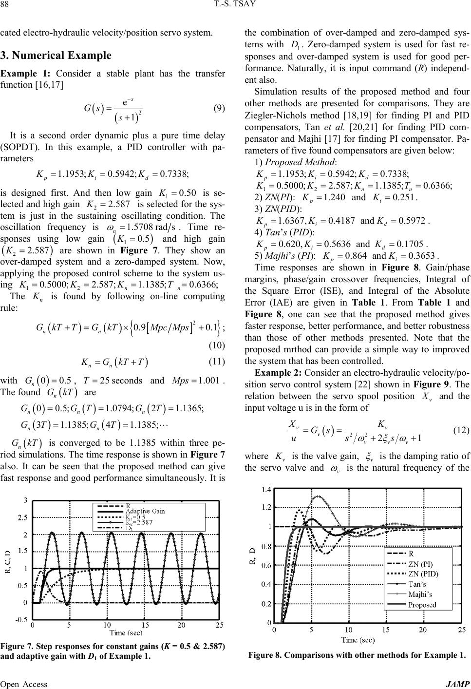

T.-S. TSAY

cated electro-hydraulic velocity/position servo system.

3. Numerical Example

Example 1: Consider a stable plant has the transfer

function [16,17]

 

Gs s



 (9)

It is a second order dynamic plus a pure time delay

(SOPDT). In this example, a PID controller with pa-

rameters

1.1953;0.5942;0.7338;

pi d

KKK 

is designed first. And then low gain 1 is se-

lected and high gain 2 is selected for the sys-

tem is just in the sustaining oscillating condition. The

oscillation frequency is

0.50K

2.587K

1.57

n08 rads





. Time re-

sponses using low gain





K

2.587;

0.5

1.1385;

K

and high gain

are shown in Figure 7. They show an

over-damped system and a zero-damped system. Now,

applying the proposed control scheme to the system us-

ing



22.587K

0.5



The

000; 0.6366;KK T

is found by following on-line computing

rule:







0.9 0.1

GkTT GkTMpcMps 





;

(10)



GkTT

(11)

with , and



00.

G525 secondsT1.001Mps



The found are



GkT



 

 

0 0.5;1.0794;21.1365;

31.1385; 41.1385;

nn n

GGTGT

GT GT

 







GkT

is converged to be 1.1385 within three pe-

riod simulations. The time response is shown in Figure 7

also. It can be seen that the proposed method can give

fast response and good performance simultaneously. It is

Figure 7. Step responses for constant gains (K = 0.5 & 2.587 )

and adaptive gain with D1 of Example 1.

the combination of over-damped and zero-damped sys-

tems with 1. Zero-damped system is used for fast re-

sponses and over-damped system is used for good per-

formance. Naturally, it is input command (R) independ-

ent also.

Simulation results of the proposed method and four

other methods are presented for comparisons. They are

Ziegler-Nichols method [18,19] for finding PI and PID

compensators, Tan et al. [20,21] for finding PID com-

pensator and Majhi [17] for finding PI compensator. Pa-

rameters of five found compensators are given below:

1) Proposed Method:

1.1953;0.5942;0.7338;

pi d

KKK





0.5000;2.587; 1.1385;

KKK

12 0.6366;





1.240

2) ZN(PI): p



and . 0.251K

3) ZN(PID):

1.6367,0.4187 and 0.5972

pi d

KK K



.

4) Tan’s (PID):

0.620,0.5636 and 0.1705

pi d

KK K





0.864 and 0.3653

5) Majhi’s (PI): pi



.

Time responses are shown in Figure 8. Gain/phase

margins, phase/gain crossover frequencies, Integral of

the Square Error (ISE), and Integral of the Absolute

Error (IAE) are given in Table 1. From Table 1 and

Figure 8, one can see that the proposed method gives

faster response, better performance, and better robustness

than those of other methods presented. Note that the

proposed mrthod can provide a simple way to improved

the system that has been controlled.

Example 2: Consider an electro-hydraulic velocity/po-

sition servo control system [22] shown in Figure 9. The

relation between the servo spool position v

and the

input voltage u is in the form of



vvv

uss





(12)

where v

is the valve gain, v



is the damping ratio of

the servo valve and v



is the natural frequency of the

Figure 8. Comparisons with other methods for Example 1.

Open Access JAMP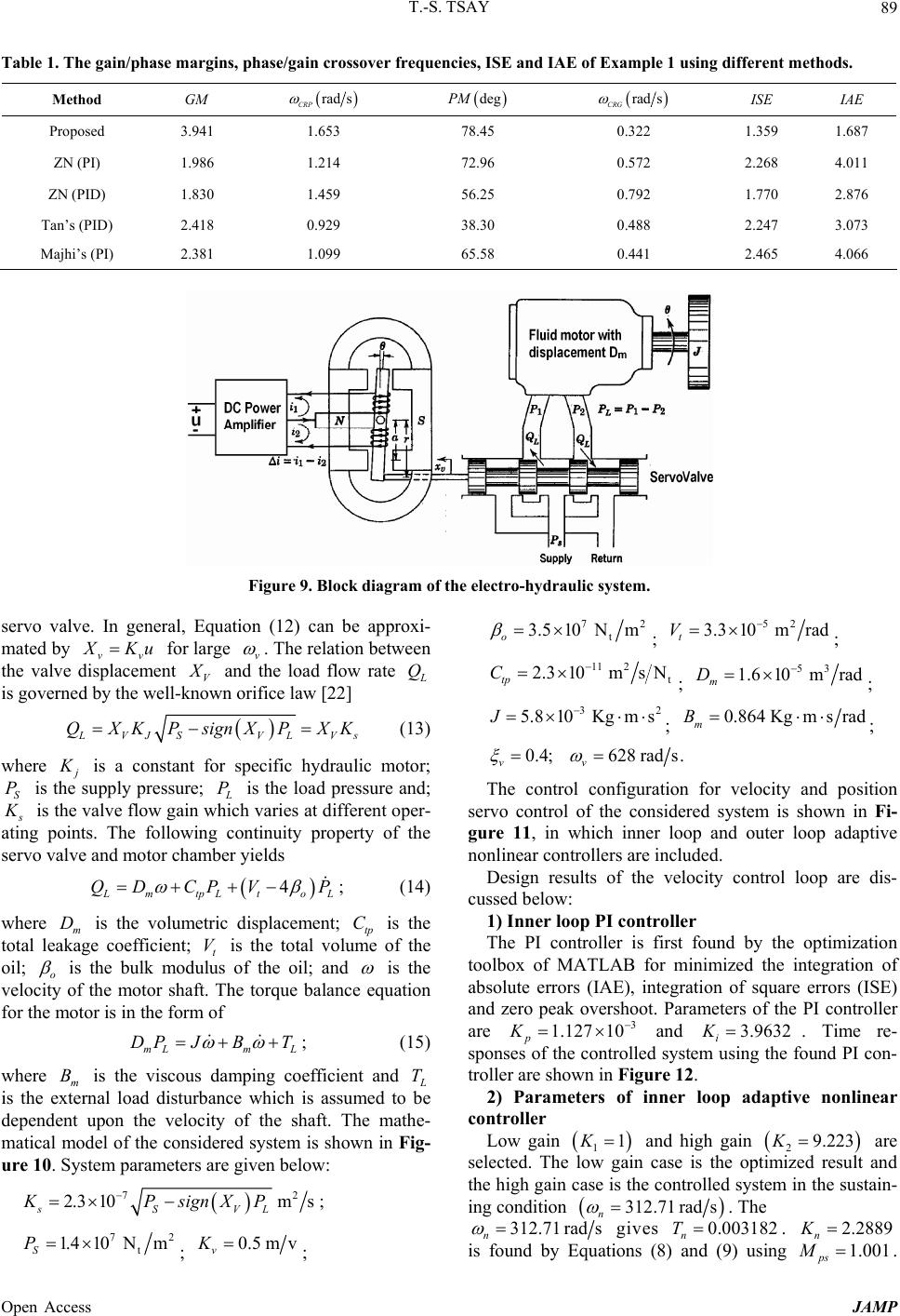

T.-S. TSAY

Open Access JAMP

Table 1. The gain/phase margins, phase/gain crossover frequencies, ISE and IAE of Example 1 using different methods.

Method GM



rad s

CRP







degPM





rad s

CRG



ISE IAE

Proposed 3.941 1.653 78.45 0.322 1.359 1.687

ZN (PI) 1.986 1.214 72.96 0.572 2.268 4.011

ZN (PID) 1.830 1.459 56.25 0.792 1.770 2.876

Tan’s (PID) 2.418 0.929 38.30 0.488 2.247 3.073

Majhi’s (PI) 2.381 1.099 65.58 0.441 2.465 4.066

Figure 9. Block diagram of the ele ctro-hydraulic system .

servo valve. In general, Equation (12) can be approxi-

mated by vv

Ku for large v



. The relation between

the valve displacement V

and the load flow rate

is governed by the well-known orifice law [22]

3.5 10Nm



 ;

3.3 10mrad

V

 ;

11 2

2.310msN

C

 ;

1.6 10mrad

D

 ;

5.810Kg m sJ





; 0.864 Kgmsrad

B

;



VJSV LVs

QXKPsignXPXK  (13)

0.4;





628 rads.





where

is a constant for specific hydraulic motor;

is the supply pressure;

P is the load pressure and;

is the valve flow gain which varies at different oper-

ating points. The following continuity property of the

servo valve and motor chamber yields

The control configuration for velocity and position

servo control of the considered system is shown in Fi-

gure 11, in which inner loop and outer loop adaptive

nonlinear controllers are included.

Design results of the velocity control loop are dis-

cussed below:





mtpLto

QD CPVP



L



; (14)

1) Inner loop PI controller

where m is the volumetric displacement; tp is the

total leakage coefficient; t is the total volume of the

oil; o



is the bulk modulus of the oil; and



is the

velocity of the motor shaft. The torque balance equation

for the motor is in the form of

The PI controller is first found by the optimization

toolbox of MATLAB for minimized the integration of

absolute errors (IAE), integration of square errors (ISE)

and zero peak overshoot. Parameters of the PI controller

are 3

1.127 10



 and . Time re-

sponses of the controlled system using the found PI con-

troller are shown in Figure 12.

3.9632

K

mLm L

DP JBT



 



; (15)

where m is the viscous damping coefficient and B

is the external load disturbance which is assumed to be

dependent upon the velocity of the shaft. The mathe-

matical model of the considered system is shown in Fig-

ure 10. System parameters are given below:

2) Parameters of inner loop adaptive nonlinear

controller

Low gain





11K



and high gain are

selected. The low gain case is the optimized result and

the high gain case is the controlled system in the sustain-

ing condition



29.223K





2.3 10ms

sSVL

KPsignXP



 ;



.71 rads312



. The

1. 410Nm

P ; 0.5 mv



;

312.71 rads



gives n

T. 0.0031822.28K





is found by Equations (8) and (9) using 1.001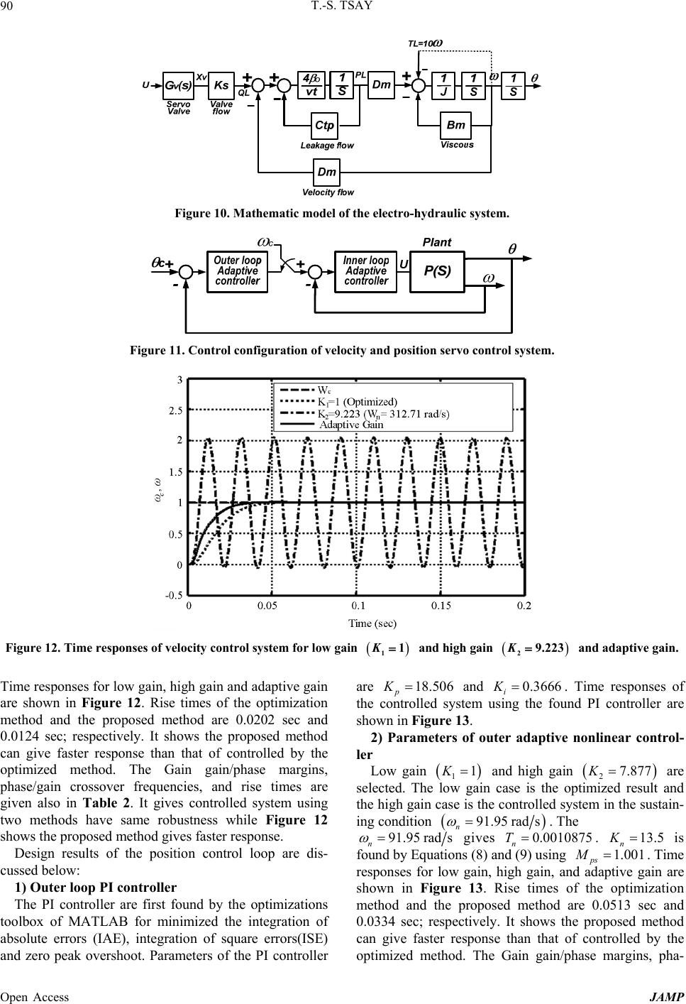



T.-S. TSAY

Figure 10. Mathematic model of the electro-hydraulic system.

Figure 11. Control configuration of velocity and position servo control system.

Figure 12. Time responses of velocity control system for low gain





K11



and high gain





K29.223 and adaptive gain.

Time responses for low gain, high gain and adaptive gain

are shown in Figure 12. Rise times of the optimization

method and the proposed method are 0.0202 sec and

0.0124 sec; respectively. It shows the proposed method

can give faster response than that of controlled by the

optimized method. The Gain gain/phase margins,

phase/gain crossover frequencies, and rise times are

given also in Table 2. It gives controlled system using

two methods have same robustness while Figure 12

shows the proposed method gives faster response.

Design results of the position control loop are dis-

cussed below:

1) Outer loop PI controller

The PI controller are first found by the optimizations

toolbox of MATLAB for minimized the integration of

absolute errors (IAE), integration of square errors(ISE)

and zero peak overshoot. Parameters of the PI controller

are 18.506



and 0.3666



. Time responses of

the controlled system using the found PI controller are

shown in Figure 13.

2) Parameters of outer adaptive nonlinear control-

ler

Low gain





11K



and high gain are

selected. The low gain case is the optimized result and

the high gain case is the controlled system in the sustain-

ing condition



27.877K





91.95 rads



. The

91.95 rads



gives n. 0.001T

n0875 13.5K





found by Equations (8) and (9) using ps

Me

responses for low gain, high gain, and adaptive gain are

shown in Figure 13. Rise times of the optimization

method and the proposed method are 0.0513 sec and

0.0334 sec; respectively. It shows the proposed method

can give faster response than that of controlled by the

optimized method. The Gain gain/phase margins, pha-

1.001 . Tim

Open Access JAMP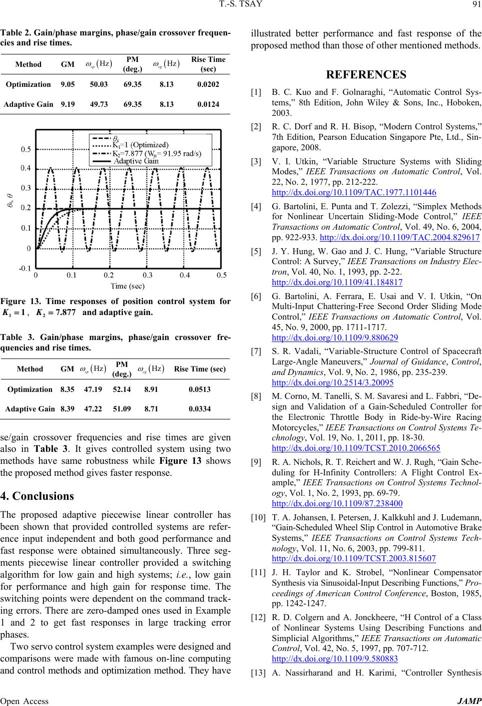

T.-S. TSAY 91

Table 2. Gain/phase margins, phase/gain cr ossover frequen-

cies and rise times.

Method GM





(deg.)





Rise Time

(sec)

Optimization 9.05 50.03 69.35 8.13 0.0202

Adaptive Gain 9.19 49.73 69.35 8.13 0.0124

Figure 13. Time responses of position control system for

, and adaptive gain. K11K27.877

Table 3. Gain/phase margins, phase/gain crossover fre-

quencies and rise times.

Method GM





(deg.)





Rise Time (sec)

Optimization 8.35 47.19 52.14 8.91 0.0513

Adaptive Gain 8.39 47.22 51.09 8.71 0.0334

se/gain crossover frequencies and rise times are given

also in Table 3. It gives controlled system using two

methods have same robustness while Figure 13 shows

the proposed method gives faster response.

4. Conclusions

The proposed adaptive piecewise linear controller has

been shown that provided controlled systems are refer-

ence input independent and both good performance and

fast response were obtained simultaneously. Three seg-

ments piecewise linear controller provided a switching

algorithm for low gain and high systems; i.e., low gain

for performance and high gain for response time. The

switching points were dependent on the command track-

ing errors. There are zero-damped ones used in Example

1 and 2 to get fast responses in large tracking error

phases.

Two servo control system examples were designed and

comparisons were made with famous on-line computing

and control methods and optimization method. They have

illustrated better performance and fast response of the

proposed method than those of other mentioned methods.

REFERENCES

[1] B. C. Kuo and F. Golnaraghi, “Automatic Control Sys-

tems,” 8th Edition, John Wiley & Sons, Inc., Hoboken,

2003.

[2] R. C. Dorf and R. H. Bisop, “Modern Control Systems,”

7th Edition, Pearson Education Singapore Pte, Ltd., Sin-

gapore, 2008.

[3] V. I. Utkin, “Variable Structure Systems with Sliding

Modes,” IEEE Transactions on Automatic Control, Vol.

22, No. 2, 1977, pp. 212-222.

http://dx.doi.org/10.1109/TAC.1977.1101446

[4] G. Bartolini, E. Punta and T. Zolezzi, “Simplex Methods

for Nonlinear Uncertain Sliding-Mode Control,” IEEE

Transactions on Automatic Control, Vol. 49, No. 6, 2004,

pp. 922-933. http://dx.doi.org/10.1109/TAC.2004.829617

[5] J. Y. Hung, W. Gao and J. C. Hung, “Variable Structure

Control: A Survey,” IEEE Transactions on Industry Elec-

tron, Vol. 40, No. 1, 1993, pp. 2-22.

http://dx.doi.org/10.1109/41.184817

[6] G. Bartolini, A. Ferrara, E. Usai and V. I. Utkin, “On

Multi-Input Chattering-Free Second Order Sliding Mode

Control,” IEEE Transactions on Automatic Control, Vol.

45, No. 9, 2000, pp. 1711-1717.

http://dx.doi.org/10.1109/9.880629

[7] S. R. Vadali, “Variable-Structure Control of Spacecraft

Large-Angle Maneuvers,” Journal of Guidance, Control,

and Dynamics, Vol. 9, No. 2, 1986, pp. 235-239.

http://dx.doi.org/10.2514/3.20095

[8] M. Corno, M. Tanelli, S. M. Savaresi and L. Fabbri, “De-

sign and Validation of a Gain-Scheduled Controller for

the Electronic Throttle Body in Ride-by-Wire Racing

Motorcycles,” IEEE Transactions on Control Systems Te-

chnology, Vol. 19, No. 1, 2011, pp. 18-30.

http://dx.doi.org/10.1109/TCST.2010.2066565

[9] R. A. Nichols, R. T. Reichert and W. J. Rugh, “Gain Sche-

duling for H-Infinity Controllers: A Flight Control Ex-

ample,” IEEE Transactions on Control Systems Technol-

ogy, Vol. 1, No. 2, 1993, pp. 69-79.

http://dx.doi.org/10.1109/87.238400

[10] T. A. Johansen, I. Petersen, J. Kalkkuhl and J. Ludemann,

“Gain-Scheduled Wheel Slip Control in Automotive Brake

Systems,” IEEE Transactions on Control Systems Tech-

nology, Vol. 11, No. 6, 2003, pp. 799-811.

http://dx.doi.org/10.1109/TCST.2003.815607

[11] J. H. Taylor and K. Strobel, “Nonlinear Compensator

Synthesis via Sinusoidal-Input Describing Functions,” Pro-

ceedings of American Control Conference, Boston, 1985,

pp. 1242-1247.

[12] R. D. Colgern and A. Jonckheere, “H Control of a Class

of Nonlinear Systems Using Describing Functions and

Simplicial Algorithms,” IEEE Transactions on Automatic

Control, Vol. 42, No. 5, 1997, pp. 707-712.

http://dx.doi.org/10.1109/9.580883

[13] A. Nassirharand and H. Karimi, “Controller Synthesis

Open Access JAMP

T.-S. TSAY

Open Access JAMP

Methodology for Multivariable Nonlinear Systems with

Application to Aerospace,” ASME Journal of Dynamic

and System Measurement Control, Vol. 126, No. 3, 2004,

pp. 595-604. http://dx.doi.org/10.1115/1.1789975

[14] A. Nassirharand and H. Karimi, “Nonlinear Controller

Synthesis Based on Inverse Describing Function Tech-

nique in the MATLAB Environment,” Advances in En-

gineering Software, Vol. 37, No. 6, 2006, pp. 370-374.

http://dx.doi.org/10.1016/j.advengsoft.2005.09.009

[15] W. K. Ho, T. H. Lee, H. P. Han and Y. Hong, “Self-Tun-

ing IMC-PID Controller with Gain and Phase Margins

Assignment,” IEEE Transactions on Control System Te ch-

nology, Vol. 9, No. 3, 2001, pp. 535-541.

[16] T. S. Tsay, “On-Line Computing of PI/Lead Compensa-

tors for Industry Processes with Gain and Phase Specifi-

cations,” Computers and Chemical Engineering, Vol. 33,

No. 9, 2009, pp. 1468-1474.

http://dx.doi.org/10.1016/j.compchemeng.2009.05.001

[17] S. Majhi, “On-Line PI Control of Stable Process,” Jour-

nal of Process Control, Vol. 15, No. 8, 2005, pp. 859-867.

http://dx.doi.org/10.1016/j.jprocont.2005.04.006

[18] J. G. Ziegler and N. B. Nichols, “Optimum Setting for

Automatic Controller,” Transactions of ASME, Vol. 65,

1942, pp. 759-768.

[19] K. J. Ǻström and T. Hägglund, “Revisting the Ziegler-

Nichols Step Responses Method for PID Control,” Jour-

nal of Process Control, Vol. 14, No. 6, 2004, pp. 635-650.

http://dx.doi.org/10.1016/j.jprocont.2004.01.002

[20] K. K. Tan, T. H Lee and X. Jiang, “Robust On-line Relay

Automatic Tuning of PID Control System,” ISA Transac-

tions, Vol. 39, 2000, pp. 219-232.

[21] K. K. Tan, T. H. Lee and X. Jiang, “On-Line Relay Iden-

tification, Assessment and Tuning of PID Controller,”

Journal of Process Control, Vol. 11, No. 5, 2001, pp. 483-

486. http://dx.doi.org/10.1016/S0959-1524(00)00012-3

[22] H. E. Merritt, “Hydraulic Control System,” John Wiley,

New York, 1967.