Flow Dynamics in Restricted Geometries: A Mathematical Concept Based on Bloch NMR Flow Equation and Boubaker Polynomial Expansion Scheme

doi:10.4236/jamp.2013.15011

Paper Menu >>

Journal Menu >>

Journal of Applied Mathematics and Physics, 2013, 1, 71-78

Published Online November 2013 (http://www.scirp.org/journal/jamp)

http://dx.doi.org/10.4236/jamp.2013.15011

Open Access JAMP

Flow Dynamics in Restricted Geometries: A Mathematical

Concept Based on Bloch NMR Flow Equation and

Boubaker Polynomial Expansion Scheme

Omotayo Bamidele Awojoyogbe1*, Oluwaseun Michael Dada1, Ka r e m Bou b ak e r2,

Omoniyi Adewale Adesola1

1Department of Physics, Federal University of Technology, Minna, Nigeria

2UPDS/ESSTT/63 Rue Sidi Jabeur 5100, Mahdia, Tunisia

Email: *[email protected]

Received August 4, 2013; revised September 25, 2013; accepted October 2, 2013

Attribution License, which permits unrestricted use, distribution, and reproduction in any medium, provided the original work is

properly cited.

ABSTRACT

Computational techniques are invaluable to the continued success and development of Magnetic Resonance Imaging

(MRI) and to its widespread applications. New processing methods are essential for addressing issues at each stage of

MRI techniques. In this study, we present new sets of non-exponential generating functions representing the NMR

transverse magnetizations and signals which are mathematically designed based on the theory and dynamics of the

Bloch NMR flow equations. These signals are functions of many spinning nuclei of materials and can be used to obtain

information observed in all flow systems. The Bloch NMR flow equations are solved using the Boubaker polynomial

expansion scheme (BPES) and analytically connect most of the experimentally valuable NMR parameters in a simpli-

fied way for general analyses of magnetic resonance imaging with adiabatic condition.

Keywords: Bloch NMR Flow Equations; Boubaker Polynomial Expansion Scheme (BPES); Magnetic Resonance

Imaging (MRI); Adiabatic Condition

1. Introduction

Flow through porous media represents a vast field of

study with many scientific and engineering applications

[1-7]. A great number of experimental and theoretical

studies on flow in restricted motion using NMR are avail-

able in the literature [1-18]. Most of these studies are based

on either numerical or approximation solutions of Bloch

NMR equations. However, it will be fundamental and ideal

if the theoretical and experimental application of MRI for

flow analysis in restricted geometry is based on the ana-

lytical solutions of Bloch NMR equations. This has been

claimed over the years to be the best approach for ob-

taining fundamental information to accurately access fluid

dynamical properties in porous media/restricted geome-

try. It is possible to derive necessary relationships ana-

lytically for free motion. However, in the case of re-

stricted motion for which porous media are defined, the

macroscopic approach becomes mathematically intracta-

ble. Thus, in general case, one is forced to use different

method to find mathematical relation for the MRI signal

in terms of NMR experimental parameters [19-21].

In this investigation, we solved the Bloch NMR flow

equation which is transformable to Bessel equation of

order zero using the Boubaker Polynomial Expansion

Scheme to obtain the NMR transverse magnetization for

the analysis of flow in anisotropic fluid flow. The rela-

tionships between fluid velocity, the NMR relaxation

rates and the path length x for cerebrospinal fluid, white

and gray matter of human cerebrum are demonstrated.

The Boubaker Polynomials Expansion Scheme BPES is a

resolution protocol which has been successfully applied

to several applied-physics and mathematics problems.

Solutions have been proposed through the BPES in many

fields such as numerical analysis [22-27], theoretical

physics [24-29], mathematical algorithms [26], heat

transfer [30,31], homodynamics [28,29], material char-

acterization [32], fuzzy systems modeling [31] and boil-

ogy [32,33].

*Corresponding author.

O. B. AWOJOYOGBE ET AL.

2. Mathematical Analysis

The BPES protocol ensures the validity of the related

boundary conditions regardless of the main features of

the equation. The BPES is mainly based on Boubaker

polynomials first derivatives properties



qxr

Bx N



;

















(1)

and



 



with: 4

nn qn

nnn n

Bx H

rr Br

Br r



































 

















(2)

In this investigation, the Boubaker Polynomials Ex-

pansion Scheme BPES has been applied to the bound-

ary-valued second order Bloch NMR flow differential

equation through setting the expression:













xr

(3)

where My(x) are the time independent NMR transverse

magnetizations, 4k are the 4k-order Boubaker poly-

nomials,





0,x1 is the normalized variable, k are

minimal positive roots, is a prefixed integer

and 0

1, ,

kkN



 are unknown pondering real coefficients.

Based on the conditions which may conform to the

real-time experimental arrangements, we obtained a sec-

ond order non homogeneous differential equation from

the Bloch NMR flow equation [34,35] at Larmor fre-

quency:







The x, y, z components (in the rotating frame) of the

magnetization of a fluid moving with spatially varying

velocity v is given by the Bloch equations which may be

written as follows:



vgradMMB x





 

T

(5)



v gradMM Bx







 

T



(6)

Subject to the following conditions:

1) Mo  Mz a situation which holds well in general and

in particular when the RF B1(x) field is strong say of the

order of 1.0 G or more.

2) Before entering signal detector coil, fluid particles

has magnetization.

Mx = 0, My = 0.

3) If B1(x) is large;





11GBx or more so that My

of the fluid bolus changes appreciably from the equilib-

rium magnetization Mo.



denotes the gyromagnetic ratio of fluid spins; 2





is the RF excitation frequency; 0



is the off-reso-

nance field in the rotating frame of reference. T1 and T2

are the spin-lattice and spin-spin relaxation times respec-

tively, the reciprocals of T1 and T2 are defined as relaxa-

tion rates. Mo is the equilibrium magnetization and RF B1

is the spatially varying magnetic field [35] which may be

designed as





Bx gx



 (7)

where g is the field gradient. Equations (5) and (6) give a

second order non-homogenous differential equation called

the Bloch NMR flow equation:

 

222

xvvT



  (8)

where

 

12 12

11 1

,TSxBx

TT TT





In NMR systems, when the RF B1 field is applied, My

has a maximum value when RF B1 has maximum ampli-

tude and Mo ≈ 0. In biological systems especially at the

molecular level we need to solve Equation (8) to provide

velocity profiles for different tissues materials such that

vnTR



 (9)



TTR



 (10)

where n is the number of pulses, TR is the repetition time.



is the time between two pulses, we write:







(11)

v gradM



 

T

(4)

For adiabatic condition, Equation (8) becomes:

Open Access JAMP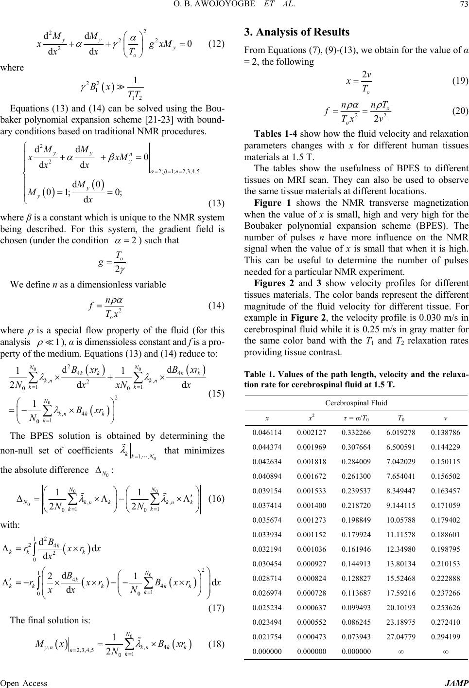

O. B. AWOJOYOGBE ET AL. 73

dd 0















(12)

where



Bx TT





Equations (13) and (14) can be solved using the Bou-

baker polynomial expansion scheme [21-23] with bound-

ary conditions based on traditional NMR procedures.

 

2;1;2,3,4,5

01; 0;

yy n

xxM















 (13)

where β is a constant which is unique to the NMR system

being described. For this system, the gradient field is

chosen (under the condition 2





) such that





We define n as a dimensionless variable

fTx





 (14)

where



is a special flow property of the fluid (for this

analysis 1



), α is dimenssioless constant and f is a pro-

perty of the medium. Equations (13) and (14) reduce to:









kk kk

kn kn

knkk

Bxr Bxr

NxN

Bxr













 









(15)

The BPES solution is obtained by determining the

non-null set of coefficients

1, ,

kkN





 that minimizes

the absolute difference :



0,,

Nknkkn











 













(16)

with:



 

kk k

kkkk k

rxrx

rxrBxr

xx N



 









 









x







(17)

The final solution is:





2,3,4,5 1

ynknk k

3. Analysis of Results

From Equations (7), (9)-(13), we obtain for the value of α

= 2, the following

 (19)

fTx v





 (20)

Tables 1-4 show how the fluid velocity and relaxation

parameters changes with x for different human tissues

materials at 1.5 T.

The tables show the usefulness of BPES to different

tissues on MRI scan. They can also be used to observe

the same tissue materials at different locations.

Figure 1 shows the NMR transverse magnetization

when the value of x is small, high and very high for the

Boubaker polynomial expansion scheme (BPES). The

number of pulses n have more influence on the NMR

signal when the value of x is small that when it is high.

This can be useful to determine the number of pulses

needed for a particular NMR experiment.

Figures 2 and 3 show velocity profiles for different

tissues materials. The color bands represent the different

magnitude of the fluid velocity for different tissue. For

example in Figure 2, the velocity profile is 0.030 m/s in

cerebrospinal fluid while it is 0.25 m/s in gray matter for

the same color band with the T1 and T2 relaxation rates

providing tissue contrast.

Table 1. Values of the path length, velocity and the relaxa-

tion rate for cerebrospinal fluid at 1.5 T.









xr

(18)

Cerebrospinal Fluid

x x2 τ = α/T0 T0 v

0.046114 0.002127 0.332266 6.019278 0.138786

0.044374 0.001969 0.307664 6.500591 0.144229

0.042634 0.001818 0.284009 7.042029 0.150115

0.040894 0.001672 0.261300 7.654041 0.156502

0.039154 0.001533 0.239537 8.349447 0.163457

0.037414 0.001400 0.218720 9.144115 0.171059

0.035674 0.001273 0.198849 10.05788 0.179402

0.033934 0.001152 0.179924 11.11578 0.188601

0.032194 0.001036 0.161946 12.34980 0.198795

0.030454 0.000927 0.144913 13.80134 0.210153

0.028714 0.000824 0.128827 15.52468 0.222888

0.026974 0.000728 0.113687 17.59216 0.237266

0.025234 0.000637 0.099493 20.10193 0.253626

0.023494 0.000552 0.086245 23.18975 0.272410

0.021754 0.000473 0.073943 27.04779 0.294199

0.000000 0.000000 0.000000 ∞ ∞

Open Access JAMP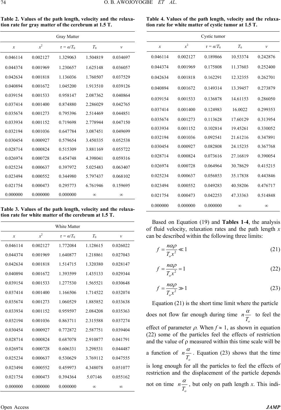

O. B. AWOJOYOGBE ET AL.

Table 2. Values of the path length, velocity and the relaxa-

tion rate for gray matter of the cerebrum at 1.5 T.

Gray Matter

x x2 τ = α/T0 T0 v

0.046114 0.002127 1.329063 1.504819 0.034697

0.044374 0.001969 1.230657 1.625148 0.036057

0.042634 0.001818 1.136036 1.760507 0.037529

0.040894 0.001672 1.045200 1.913510 0.039126

0.039154 0.001533 0.958147 2.087362 0.040864

0.037414 0.001400 0.874880 2.286029 0.042765

0.035674 0.001273 0.795396 2.514469 0.044851

0.033934 0.001152 0.719698 2.778944 0.047150

0.032194 0.001036 0.647784 3.087451 0.049699

0.030454 0.000927 0.579654 3.450335 0.052538

0.028714 0.000824 0.515309 3.881169 0.055722

0.026974 0.000728 0.454748 4.398041 0.059316

0.025234 0.000637 0.397972 5.025483 0.063407

0.023494 0.000552 0.344980 5.797437 0.068102

0.021754 0.000473 0.295773 6.761946 0.159695

0.000000 0.000000 0.000000 ∞ ∞

Table 3. Values of the path length, velocity and the relaxa-

tion rate for white matter of the cerebrum at 1.5 T.

White Matter

x x2 τ = α/T0 T0 v

0.046114 0.002127 1.772084 1.128615 0.026022

0.044374 0.001969 1.640877 1.218861 0.027043

0.042634 0.001818 1.514715 1.320380 0.028147

0.040894 0.001672 1.393599 1.435133 0.029344

0.039154 0.001533 1.277530 1.565521 0.030648

0.037414 0.001400 1.166506 1.714522 0.032074

0.035674 0.001273 1.060529 1.885852 0.033638

0.033934 0.001152 0.959597 2.084208 0.035363

0.032194 0.001036 0.863711 2.315588 0.037274

0.030454 0.000927 0.772872 2.587751 0.039404

0.028714 0.000824 0.687078 2.910877 0.041791

0.026974 0.000728 0.606331 3.298531 0.044487

0.025234 0.000637 0.530629 3.769112 0.047555

0.023494 0.000552 0.459973 4.348078 0.051077

0.021754 0.000473 0.394364 5.07146 0.055162

0.000000 0.000000 0.000000 ∞ ∞

Table 4. Values of the path length, velocity and the relaxa-

tion rate for white matter of cystic tumor at 1.5 T.

Cystic tumor

x x2 τ = α/T0 T0 v

0.046114 0.002127 0.189866 10.53374 0.242876

0.044374 0.001969 0.175808 11.37603 0.252400

0.042634 0.001818 0.162291 12.32355 0.262701

0.040894 0.001672 0.149314 13.39457 0.273879

0.039154 0.001533 0.136878 14.61153 0.286050

0.037414 0.001400 0.124983 16.0022 0.299353

0.035674 0.001273 0.113628 17.60129 0.313954

0.033934 0.001152 0.102814 19.45261 0.330052

0.032194 0.001036 0.092541 21.61216 0.347891

0.030454 0.000927 0.082808 24.15235 0.367768

0.028714 0.000824 0.073616 27.16819 0.390054

0.026974 0.000728 0.064964 30.78629 0.415215

0.025234 0.000637 0.056853 35.17838 0.443846

0.023494 0.000552 0.049283 40.58206 0.476717

0.021754 0.000473 0.042253 47.33363 0.514848

0.000000 0.000000 0.000000 ∞ ∞

Based on Equation (19) and Tables 1-4, the analysis

of fluid velocity, relaxation rates and the path length x

can be described within the following three limits:

fTx



 (21)

fTx





 (22)

fTx



 (23)

Equation (21) is the short time limit where the particle

does not flow far enough during time



to feel the

effect of parameter



. When f  1, as shown in equation

(22) some of the particles feel the effects of restriction

and the value of  measured within this time scale will be

a function of



. Equation (23) shows that the time

is long enough for all the particles to feel the effects of

restriction and the displacement of the particle depends

not on time



, but only on path length x. This indi-

Open Access JAMP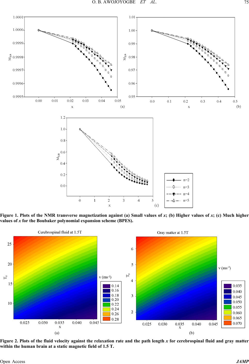

O. B. AWOJOYOGBE ET AL.

Open Access JAMP

Figure 1. Plots of the NMR transverse magnetization against (a) Small values of x; (b) Higher values of x; (c) Much higher

values of x for the Boubaker polynomial expansion scheme (BP ES).

(a) (b)

Figure 2. Plots of the fluid velocity against the relaxation rate and the path length x for cerebrospinal fluid and gray matter

within the human brain at a static magnetic field of 1.5 T.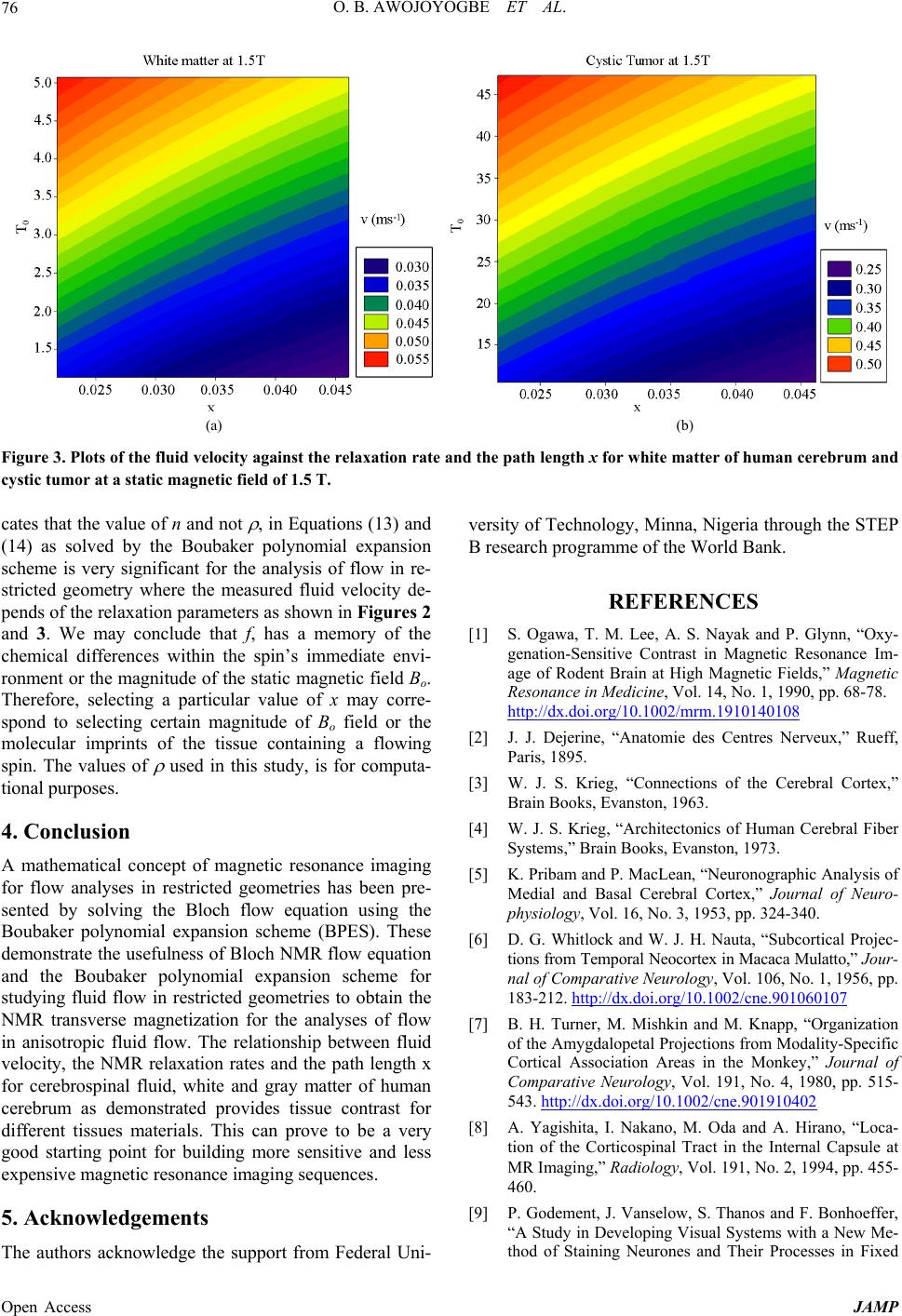

O. B. AWOJOYOGBE ET AL.

(a) (b)

Figure 3. Plots of the fluid velocity against the relaxation rate and the path length x for white matter of human cerebrum and

cystic tumor at a static magnetic field of 1.5 T.

cates that the value of n and not



, in Equations (13) and

(14) as solved by the Boubaker polynomial expansion

scheme is very significant for the analysis of flow in re-

stricted geometry where the measured fluid velocity de-

pends of the relaxation parameters as shown in Figures 2

and 3. We may conclude that f, has a memory of the

chemical differences within the spin’s immediate envi-

ronment or the magnitude of the static magnetic field Bo.

Therefore, selecting a particular value of x may corre-

spond to selecting certain magnitude of Bo field or the

molecular imprints of the tissue containing a flowing

spin. The values of



used in this study, is for computa-

tional purposes.

4. Conclusion

A mathematical concept of magnetic resonance imaging

for flow analyses in restricted geometries has been pre-

sented by solving the Bloch flow equation using the

Boubaker polynomial expansion scheme (BPES). These

demonstrate the usefulness of Bloch NMR flow equation

and the Boubaker polynomial expansion scheme for

studying fluid flow in restricted geometries to obtain the

NMR transverse magnetization for the analyses of flow

in anisotropic fluid flow. The relationship between fluid

velocity, the NMR relaxation rates and the path length x

for cerebrospinal fluid, white and gray matter of human

cerebrum as demonstrated provides tissue contrast for

different tissues materials. This can prove to be a very

good starting point for building more sensitive and less

expensive magnetic resonance imaging sequences.

5. Acknowledgements

The authors acknowledge the support from Federal Uni-

versity of Technology, Minna, Nigeria through the STEP

B research programme of the World Bank.

REFERENCES

[1] S. Ogawa, T. M. Lee, A. S. Nayak and P. Glynn, “Oxy-

genation-Sensitive Contrast in Magnetic Resonance Im-

age of Rodent Brain at High Magnetic Fields,” Magnetic

Resonance in Medicine, Vol. 14, No. 1, 1990, pp. 68-78.

http://dx.doi.org/10.1002/mrm.1910140108

[2] J. J. Dejerine, “Anatomie des Centres Nerveux,” Rueff,

Paris, 1895.

[3] W. J. S. Krieg, “Connections of the Cerebral Cortex,”

Brain Books, Evanston, 1963.

[4] W. J. S. Krieg, “Architectonics of Human Cerebral Fiber

Systems,” Brain Books, Evanston, 1973.

[5] K. Pribam and P. MacLean, “Neuronographic Analysis of

Medial and Basal Cerebral Cortex,” Journal of Neuro-

physiology, Vol. 16, No. 3, 1953, pp. 324-340.

[6] D. G. Whitlock and W. J. H. Nauta, “Subcortical Projec-

tions from Temporal Neocortex in Macaca Mulatto,” Jour-

nal of Comparative Neurology, Vol. 106, No. 1, 1956, pp.

183-212. http://dx.doi.org/10.1002/cne.901060107

[7] B. H. Turner, M. Mishkin and M. Knapp, “Organization

of the Amygdalopetal Projections from Modality-Specific

Cortical Association Areas in the Monkey,” Journal of

Comparative Neurology, Vol. 191, No. 4, 1980, pp. 515-

543. http://dx.doi.org/10.1002/cne.901910402

[8] A. Yagishita, I. Nakano, M. Oda and A. Hirano, “Loca-

tion of the Corticospinal Tract in the Internal Capsule at

MR Imaging,” Radiology, Vol. 191, No. 2, 1994, pp. 455-

460.

[9] P. Godement, J. Vanselow, S. Thanos and F. Bonhoeffer,

“A Study in Developing Visual Systems with a New Me-

thod of Staining Neurones and Their Processes in Fixed

Open Access JAMP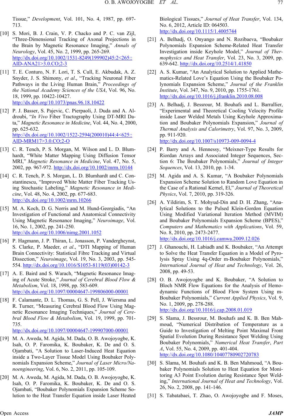

O. B. AWOJOYOGBE ET AL. 77

Tissue,” Development, Vol. 101, No. 4, 1987, pp. 697-

713.

[10] S. Mori, B. J. Crain, V. P. Chacko and P. C. van Zijl,

“Three-Dimensional Tracking of Axonal Projections in

the Brain by Magnetic Resonance Imaging,” Annals of

Neurology, Vol. 45, No. 2, 1999, pp. 265-269.

http://dx.doi.org/10.1002/1531-8249(199902)45:2<265::

AID-ANA21>3.0.CO;2-3

[11] T. E. Conturo, N. F. Lori, T. S. Cull, E. Akbudak, A. Z.

Snyder, J. S. Shimony, et al., “Tracking Neuronal Fiber

Pathways in the Living Human Brain,” Proceedings of

the National Academy Sciences of the USA, Vol. 96, No.

18, 1999, pp. 10422-10427.

http://dx.doi.org/10.1073/pnas.96.18.10422

[12] P. J. Basser, S. Pajevic, C. Pierpaoli, J. Duda and A. Al-

droubi, “In Vivo Fiber Tractography Using DT-MRI Da-

ta,” Magnetic Resonance in Medicine, Vol. 44, No. 4, 2000,

pp. 625-632.

http://dx.doi.org/10.1002/1522-2594(200010)44:4<625::

AID-MRM17>3.0.CO;2-O

[13] C. R. Tench, P. S. Morgan, M. Wilson and L. D. Blum-

hardt, “White Matter Mapping Using Diffusion Tensor

MRI,” Magnetic Resonance in Medicine, Vol. 47, No. 5,

2002, pp. 967-972. http://dx.doi.org/10.1002/mrm.10144

[14] C. R. Tench, P. S. Morgan, L. D. Blumhardt and C. Con-

stantinescu, “Improved White Matter Fiber Tracking Us-

ing Stochastic Labeling,” Magnetic Resonance in Medi-

cine, Vol. 48, No. 4, 2002, pp. 677-683.

http://dx.doi.org/10.1002/mrm.10266

[15] M. A. Koch, D. G. Norris and M. Hund-Georgiadis, “An

Investigation of Functional and Anatomical Connectivity

Using Magnetic Resonance Imaging,” Neuroimage, Vol.

16, No. 1, 2002, pp. 241-250.

http://dx.doi.org/10.1006/nimg.2001.1052

[16] P. Hagmann, J. P. Thiran, L. Jonasson, P. Vandergheynst,

S. Clarke, P. Maeder, et al., “DTI Mapping of Human

Brain Connectivity: Statistical Fibre Tracking and Virtual

Dissection,” Neuroimage, Vol. 19, No. 3, 2003, pp. 545-

554. http://dx.doi.org/10.1016/S1053-8119(03)00142-3

[17] A. E. Baird and S. Warach, “Magnetic Resonance Imag-

ing of Acute Stroke,” Journal of Cerebral Blood Flow &

Metabolism, Vol. 18, 1998, pp. 583-609.

http://dx.doi.org/10.1097/00004647-199806000-00001

[18] F. Calamante, D. L. Thomas, G. S. Pell, J. Wiersma and

R. Turner, “Measuring Cerebral Blood Flow Using Mag-

netic Resonance Imaging Techniques,” Journal of Cere-

bral Blood Flow & Metabolism, Vol. 19, 1999, pp. 701-

735.

http://dx.doi.org/10.1097/00004647-199907000-00001

[19] M. A. Aweda, M. Agida, M. Dada, O. B. Awojoyogbe, K.

Isah, O. P. Faromika, K. Boubaker, K. De and O. S.

Ojambati, “A Solution to Laser-Induced Heat Equation

inside a Two-Layer Tissue Model Using Boubaker Poly-

nomials Expansion Scheme,” Journal of Laser Micro/Na-

noengineering, Vol. 6, No. 2, 2011, pp. 105-109.

[20] M. A. Aweda, M. Agida, M. Dada, O. B. Awojoyogbe, K.

Isah, O. P. Faromika, K. Boubaker, K. De and O. S.

Ojambati, “Boubaker Polynomials Expansion Scheme So-

lution to the Heat Transfer Equation inside Laser Heated

Biological Tissues,” Journal of Heat Transfer, Vol. 134,

No. 6, 2012, Article ID: 064503.

http://dx.doi.org/10.1115/1.4005744

[21] A. Belhadj, O. Onyango and N. Rozibaeva, “Boubaker

Polynomials Expansion Scheme-Related Heat Transfer

Investigation inside Keyhole Model,” Journal of Ther-

mophysics and Heat Transfer, Vol. 23, No. 3, 2009, pp.

639-642. http://dx.doi.org/10.2514/1.41850

[22] A. S. Kumar, “An Analytical Solution to Applied Mathe-

matics-Related Love’s Equation Using the Boubaker Po-

lynomials Expansion Scheme,” Journal of the Franklin

Institute, Vol. 347, No. 9, 2010, pp. 1755-1761.

http://dx.doi.org/10.1016/j.jfranklin.2010.08.008

[23] A. Belhadj, J. Bessrour, M. Bouhafs and L. Barrallier,

“Experimental and Theoretical Cooling Velocity Profile

inside Laser Welded Metals Using Keyhole Approxima-

tion and Boubaker Polynomials Expansion,” Journal of

Thermal Analysis and Calorimetry, Vol. 97, No. 3, 2009,

pp. 911-920.

http://dx.doi.org/10.1007/s10973-009-0094-4

[24] P. Barry and A. Hennessy, “Meixner-Type Results for

Riordan Arrays and Associated Integer Sequences, Sec-

tion 6: The Boubaker Polynomials,” Journal of Integer

Sequences, Vol. 13, 2010, pp. 1-34.

[25] M. Agida and A. S. Kumar, “A Boubaker Polynomials

Expansion Scheme Solution to Random Love Equation in

the Case of a Rational Kernel, El,” Journal of Theoretical

Physics, Vol. 7, 2010, pp. 319-326.

[26] A. Yildirim, S. T. Mohyud-Din and D. H. Zhang, “Ana-

lytical Solutions to the Pulsed Klein-Gordon Equation

Using Modified Variational Iteration Method (MVIM)

and Boubaker Polynomials Expansion Scheme (BPES),”

Computers and Mathematics with Applications, Vol. 59,

No. 8, 2010, pp. 2473-2477.

http://dx.doi.org/10.1016/j.camwa.2009.12.026

[27] J. Ghanouchi, H. Labiadh and K. Boubaker, “An Attempt

to Solve the Heat Transfer Equation in a Model of Pyro-

lysis Spray Using 4q-Order m-Boubaker Polynomials,”

International Journal of Heat and Technology, Vol. 26,

2008, pp. 49-53.

[28] O. B. Awojoyogbe and K. Boubaker, “A Solution to

Bloch NMR Flow Equations for the Analysis of Hemo-

dynamic Functions of Blood Flow System Using m-

Boubaker Polynomials,” Current Applied Physics, Vol. 9,

No. 1, 2009, pp. 278-288.

http://dx.doi.org/10.1016/j.cap.2008.01.019

[29] S. Slama, J. Bessrour, M. Bouhafs and K. B. Ben Mah-

moud, “Numerical Distribution of Temperature as a

Guide to Investigation of Melting Point Maximal Front

Spatial Evolution During Resistance Spot Welding Using

Boubaker Polynomials,” Numerical Heat Transfer, Part

A, Vol. 55, No. 4, 2009, pp. 401-404.

http://dx.doi.org/10.1080/10407780902720783

[30] S. Slama, M. Bouhafs and K. B. Ben Mahmoud, “A Bou-

baker Polynomials Solution to Heat Equation for Moni-

toring A3 Point Evolution during Resistance Spot Weld-

ing,” International Journal of Heat and Technology, Vol.

26, No. 2, 2008, pp. 141-146.

[31] S. Tabatabaei, T. Zhao, O. Awojoyogbe and F. Moses,

Open Access JAMP

O. B. AWOJOYOGBE ET AL.

Open Access JAMP

“Cut-off Cooling Velocity Profiling inside a Keyhole Mo-

del Using the Boubaker Polynomials Expansion Scheme,”

International Journal of Heat and Mass Transfer, Vol. 45,

No. 10, 2009, pp. 1247-1255.

http://dx.doi.org/10.1007/s00231-009-0493-x

[32] S. Fridjine and M. Amlouk, “A New Parameter: An

ABACUS for Optimizing Functional Materials Using the

Boubaker Polynomials Expansion Scheme,” Modern Phy-

sics Letters B, Vol. 23, No. 17, 2009, pp. 2179-2182.

http://dx.doi.org/10.1142/S0217984909020321

[33] A. Milgram, “The Stability of the Boubaker Polynomials

Expansion Scheme (BPES)-Based Solution to Lotka-Vol-

terra Problem,” Journal of Theoretical Biology, Vol. 271,

No. 1, 2011, pp. 157-158.

http://dx.doi.org/10.1016/j.jtbi.2010.12.002

[34] O. B. Awojoyogbe, “Analytical Solution of the Time De-

pendent Bloch NMR Equations: A Translational Mecha-

nical Approach,” Physica A, Vol. 339, No. 3-4, 2004, pp.

437-460. http://dx.doi.org/10.1016/j.physa.2004.03.061

[35] O. B. Awojoyogbe, O. M. Dada, O. P. Faromika and O. E.

Dada, “Mathematical Concept of the Bloch Flow Equa-

tions for General Magnetic Resonance Imaging: A Re-

view,” Concepts in Magnetic Resonance Part A, Vol. 38A,

No. 3, 2011, pp. 85-101.

http://dx.doi.org/10.1002/cmr.a.20210