Simulation of Fault Arc Using Conventional Arc Models

doi:10.4236/epe.2013.54B160

Paper Menu >>

Journal Menu >>

Energy and Power Engineering, 2013, 5, 833-837

doi:10.4236/epe.2013.54B160 Published Online July 2013 (http://www.scirp.org/journal/epe)

Simulation of Fault Arc Using Conventional Arc Models

Ling Yuan, Lin Sun, Huaren Wu

School of Electrical and Automation Engineering, Nanjing Normal University, Nanjing, China

Email: [email protected]

Received April, 2013

ABSTRACT

Conventional arc models are usually used to research the interaction between switching arc and circuit. It is important to

simulate the fault arc for arc flash calculations, choice of electrical equipments and power system protection. This paper

investigates several conventional arc models for calculating the fault arcing current. Simulation results show that con-

ventional arc models can be used to simulate the fault arc if the parameters of arc models are given properly. This paper

provides the parameters of 5 popular arc models and describes the simulation results of the fault arc.

Keywords: Arc; Arc Flash; Arc Model; Plasma; Power System

1. Introduction

Short circuit in power systems is serious fault. The short

circuit current must be calculated for the choice of elec-

trical equipments and the setting of power system protec-

tion. An arc presents usually at the fault location in pow-

er systems. The fault arc could destroy electrical equip-

ment and threaten human life. It is important to calculate

the arc fault current for reducing loss.

An arc model must be used for calculation of the arc

fault current. There are a lot of arc models for describing

the arc. Arc models can be classified in three groups:

physical models, black box models and models based on

graphics and diagrams. Black box models describe only

the relation between input and output signals. Black box

models define the interaction between the arc and the

electrical circuit during the fault. In black box models,

the arc is described by one differential equation or sev-

eral differential equations relating the arc conductance

which describes the energy balance of the arc column.

Cassie arc model was presented by Cassie in 1939 [1].

Cassie assumed that the arc has a fixed temperature being

cooled by forced convection. This implies that the

cross-section area of the arc is proportional to the current

and that the voltage over the arc is constant. Cassie arc

model is suitable for arcs with high currents.

Mayr arc model was introduced in 1943 [2, 3]. Mayr

assumed that power losses are caused by thermal con-

duction and the arc conductance is dependent on tem-

perature. The cross-section area of the arc is assumed

constant. Mayr arc model is fit for currents near zero.

Schwarz developed a modified Mayr arc model in

1971[4]. The time constant and the cooling power in the

model are dependent on the arc conductance [5].

Habedank arc model is a series connection of a Cassie

and Mayr arc model [6]. It is suitable for arcs with high

currents and for currents near zero.

A modified Mayr arc model was presented in 1992 [7].

The cooling power in the model is current-dependent.

Schavemaker arc model is also a modified Mayr arc

model with a constant time parameter [8]. The cooling

power in the model is a function of the electrical power

input.

The above-mentioned arc models are black box mod-

els, that is, conventional arc models. They are usually

used to research the interaction between switching arc

and circuit during the interruption process of circuit

breakers. The characteristics of the fault arc are different

from that of the switching arc. This paper describes the

simulation methods of the fault arc using conventional

arc models. First of all the arcing fault was tested in the

high-power test laboratory and the arc voltage and the arc

current are depicted. Then 5 arc models are investigated

and their parameters are determined for simulation of the

fault arc. Conventional arc models can be used to simu-

late the fault arc.

2. Simulation of Fault Arc

Short circuit was tested in the high-power test laboratory.

The simplified laboratory test circuit is shown in Figure

1. The supply voltage is 400V.

The arc was initiated by means of a fuse wire between

2 electrodes. The arc voltage and the arc current were

recorded with the sampling frequency of 40 kHz and are

depicted in Figure 2. Figure 2 shows that arc voltage

and arc current are in phase and the arc is resistive. The

arc voltage ought to be represented for simulation the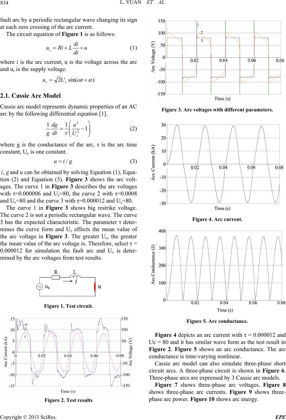

L. YUAN ET AL.

834

fault arc by a periodic rectangular wave changing its sign

at each zero crossing of the arc current.

The circuit equation of Figure 1 is as follows:

sdi

uRiL u

 

(1)

where i is the arc current, u is the voltage across the arc

and us is the supply voltage.

2sin( )

uU t







2.1. Cassie Arc Model

Cassie arc model represents dynamic properties of an AC

arc by the following differential equation [1].

11 1

dg u

gdt U













(2)

where g is the conductance of the arc, τ is the arc time

constant, Uc is one constant.

/uig (3)

,andig ucan be obtained by solving Equation (1), Equa-

tion (2) and Equation (3). Figure 3 shows the arc volt-

ages. The curve 1 in Figure 3 describes the arc voltages

with τ=0.000006 and Uc=80, the curve 2 with τ=0.0008

and Uc=80 and the curve 3 with τ=0.000012 and Uc=80.

The curve 1 in Figure 3 shows big restrike voltage.

The curve 2 is not a periodic rectangular wave. The curve

3 has the expected characteristic. The parameter τ deter-

mines the curve form and Uc effects the mean value of

the arc voltage in Figure 3. The greater Uc, the greater

the mean value of the arc voltage is. Therefore, select τ =

0.000012 for simulation the fault arc and Uc is deter-

mined by the arc voltages from test results.

Figure 1. Test circuit.

Figure 2. Test results

Figure 3. Arc voltages with different parameters.

Figure 4. Arc current.

Figure 5. Arc conductance.

Figure 4 depicts an arc current with τ = 0.000012 and

Uc = 80 and it has similar wave form as the test result in

Figure 2. Figure 5 shows an arc conductance. The arc

conductance is time-varying nonlinear.

Cassie arc model can also simulate three-phase short

circuit arcs. A three-phase circuit is shown in Figure 6.

Three-phase arcs are expressed by 3 Cassie arc models.

Figure 7 shows three-phase arc voltages. Figure 8

shows three-phase arc currents. Figure 9 shows three-

phase arc power. Figure 10 shows arc energy.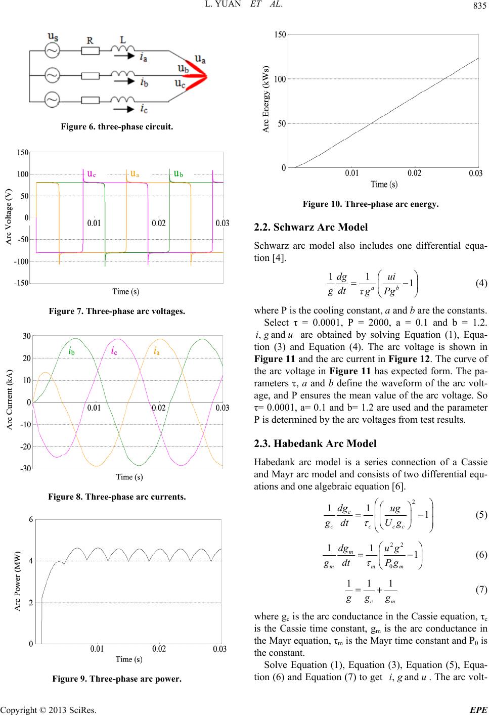

L. YUAN ET AL. 835

Figure 6. three-phase circuit.

Figure 7. Three-phase arc voltages.

Figure 8. Three-phase arc currents.

Figure 9. Three-phase arc power.

Figure 10. Three-phase arc energy.

2.2. Schwarz Arc Model

Schwarz arc model also includes one differential equa-

tion [4].

11 1

dg ui

gdt gPg















(4)

where P is the cooling constant, a and b are the constants.

Select τ = 0.0001, P = 2000, a = 0.1 and b = 1.2.

are obtained by solving Equation (1), Equa-

tion (3) and Equation (4). The arc voltage is shown in

Figure 11 and the arc current in Figure 12. The curve of

the arc voltage in Figure 11 has expected form. The pa-

rameters τ, a and b define the waveform of the arc volt-

age, and P ensures the mean value of the arc voltage. So

τ= 0.0001, a= 0.1 and b= 1.2 are used and the parameter

P is determined by the arc voltages from test results.

,andig u

2.3. Habedank Arc Model

Habedank arc model is a series connection of a Cassie

and Mayr arc model and consists of two differential equ-

ations and one algebraic equation [6].

11 1

cccc

dg ug

gdtUg



















(5)

11 1

mmm

dg ug

gdt Pg















(6)

11 1

 (7)

where gc is the arc conductance in the Cassie equation, τc

is the Cassie time constant, gm is the arc conductance in

the Mayr equation, τm is the Mayr time constant and P0 is

the constant.

Solve Equation (1), Equation (3), Equation (5), Equa-

tion (6) and Equation (7) to get . The arc volt-

,andig u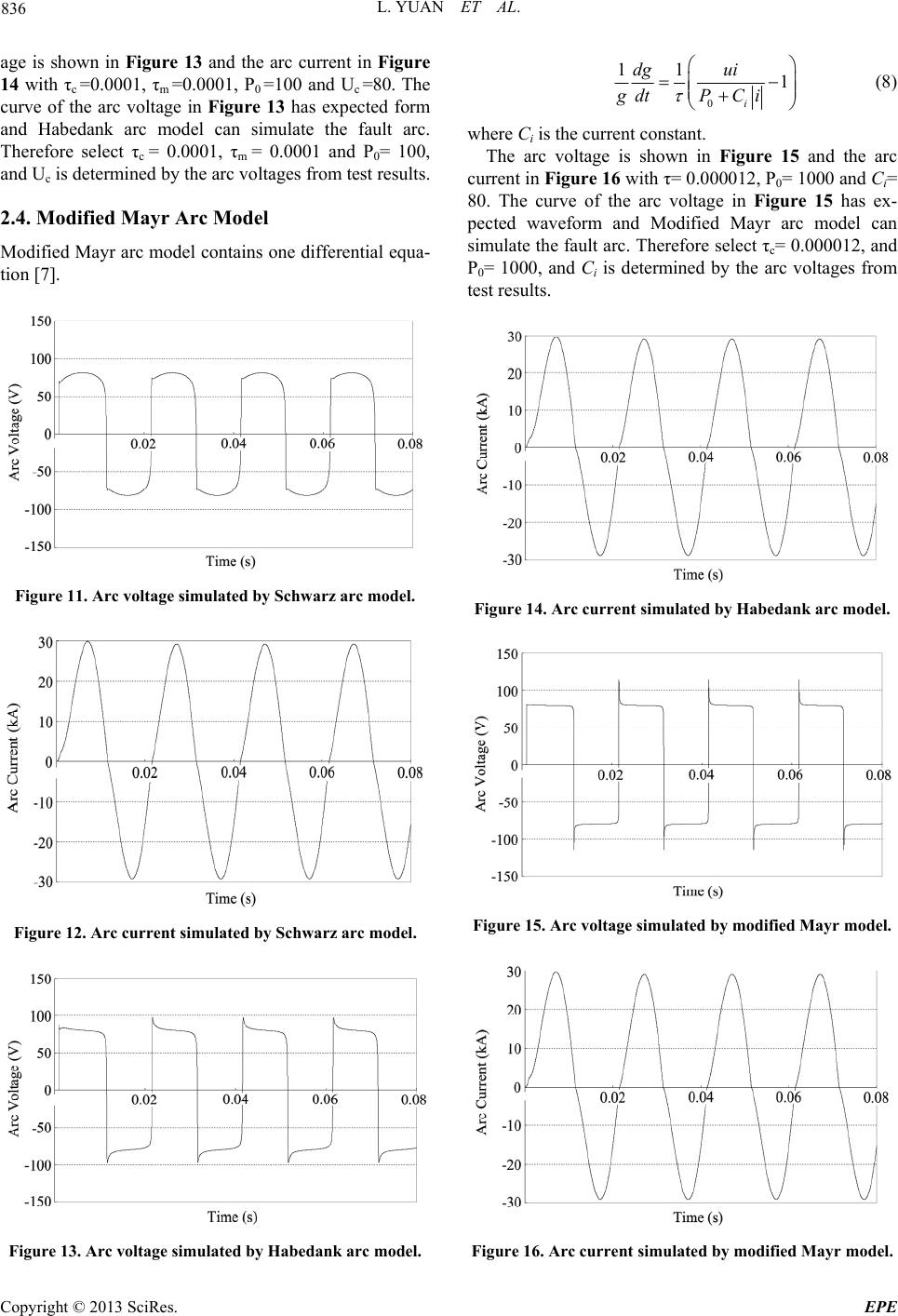

L. YUAN ET AL.

836

age is shown in Figure 13 and the arc current in Figure

14 with τc =0.0001, τm =0.0001, P0 =100 and Uc =80. The

curve of the arc voltage in Figure 13 has expected form

and Habedank arc model can simulate the fault arc.

Therefore select τc = 0.0001, τm = 0.0001 and P0= 100,

and Uc is determined by the arc voltages from test results.

2.4. Modified Mayr Arc Model

Modified Mayr arc model contains one differential equa-

tion [7].

Figure 11. Arc voltage simulated by Schwarz arc model.

Figure 12. Arc current simulated by Schwarz arc model.

Figure 13. Arc voltage simulated by Habedank arc model.

11 1

dg ui

gdtP Ci

















(8)

where Ci is the current constant.

The arc voltage is shown in Figure 15 and the arc

current in Figure 16 with τ= 0.000012, P0= 1000 and Ci=

80. The curve of the arc voltage in Figure 15 has ex-

pected waveform and Modified Mayr arc model can

simulate the fault arc. Therefore select τc= 0.000012, and

P0= 1000, and Ci is determined by the arc voltages from

test results.

Figure 14. Arc current simulated by Habedank arc model.

Figure 15. Arc voltage simulated by modified Mayr model.

Figure 16. Arc current simulated by modified Mayr model.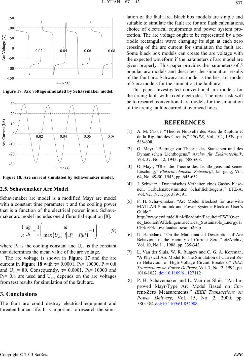

L. YUAN ET AL.

837

Figure 17. Arc voltage simulated by Schavemaker model.

Figure 18. Arc current simulated by Schavemaker model.

2.5. Schavemaker Arc Model

Schavemaker arc model is a modified Mayr arc model

with a constant time parameter τ and the cooling power

that is a function of the electrical power input. Schave-

maker arc model includes one differential equation [8].



11 1

max ,

arc

dg ui

gdt UiPPui

























(9)

where P1 is the cooling constant and Uarc is the constant

that determines the mean value of the arc voltage.

The arc voltage is shown in Figure 17 and the arc

current in Figure 18 with τ= 0.0001, P0= 10000, P1= 0.8

and Uarc= 80. Consequently, τ= 0.0001, P0= 10000 and

P1= 0.8 are used and Uarc depends on the arc voltages

from test results for simulation of the fault arc.

3. Conclusions

The fault arc could destroy electrical equipment and

threaten human life. It is important to research the simu-

lation of the fault arc. Black box models are simple and

suitable to simulate the fault arc for arc flash calculations,

choice of electrical equipments and power system pro-

tection. The arc voltage ought to be represented by a pe-

riodic rectangular wave changing its sign at each zero

crossing of the arc current for simulation the fault arc.

Some black box models can create the arc voltage with

the expected waveform if the parameters of arc model are

given properly. This paper provides the parameters of 5

popular arc models and describes the simulation results

of the fault arc. Schwarz arc model is the best arc model

of 5 arc models for the simulation the fault arc.

This paper investigated conventional arc models for

the arcing fault with fixed electrodes. The next task will

be to research conventional arc models for the simulation

of the arcing fault occurred at overhead lines.

REFERENCES

[1] A. M. Cassie, “Theorie Nouvelle des Arcs de Rupture et

de la Rigidité des Circuits,” CIGRE, Vol. 102, 1939, pp.

588-608.

[2] O. Mayr, “Beitrage zur Theorie des Statischen und des

Dynamischen Lichtbogens,” Archiv für Elektrotechnik,

Vol. 37, No. 12, 1943, pp. 588-608.

[3] O. Mayr, “Über die Theorie des Lichtbogens und seiner

Löschung,” Elektrotechnische Zeitschrift, Jahrgang, Vol.

64, No. 49-50, 1943, pp. 645-652.

[4] J. Schwarz, “Dynamisches Verhalten eines Gasbe- blase-

nen, Turbulenzbestimmten Schaltlichtbogens,” ETZ-A,

Vol. 92, 1971, pp. 389-391.

[5] P. H. Schavemaker, “Arc Model Blockset for use with

MATLAB Simulink and Power System: Blockset-User’s

Guide,”

http://www.ewi.tudelft.nl/fileadmin/Faculteit/EWI/Over_

de_faculteit/Afdelingen/Electrical_Sustainable_Energy/H

CPS/EPS/downloads/doc/amb2.zip

[6] U. Habedank, “On the Mathematical Description of Arc

Behaviour in the Vicinity of Current Zero,” etzArchiv,

Vol. 10, No.11, 1988, pp. 339-343.

[7] L. Van der Sluis, W. R. Rutgers and C. G. A. Koreman,

“A Physical Arc Model for the Simulation of Current Ze-

ro Behaviour of High-Voltage Circuit Breakers,” IEEE

Transactions on Power Delivery, Vol. 7, No. 2, 1992, pp.

1016-1022. doi:10.1109/61.127112

[8] P. H. Schavemaker and L. Van der Sluis, “An Im-

proved Mayr-Type Arc Model Based on Cur-

rent-Zero Measurements,” IEEE Transactions on

Power Delivery, Vol. 15, No. 2, 2000, pp.

580-584.doi:10.1109/61.852988