Pressure-Driven Demand and Leakage Simulation for Pipe Networks Using Differential Evolution

doi:10.4236/wjet.2013.13008

Paper Menu >>

Journal Menu >>

World Journal of Engineering and Technology, 2013, 1, 49-58

Published Online November 2013 (http://www.scirp.org/journal/wjet)

http://dx.doi.org/10.4236/wjet.2013.13008

Open Access WJET

Pressure-Driven Demand and Leakage Simulation for Pipe

Networks Using Differential Evolution

Naser Moosavian, Mohammad Reza Jaefarzadeh

Department of Civil Engineering, Ferdowsi University of Mashhad, Mashhad, Iran.

Email: [email protected]

Received September 1st, 2013; revised October 2nd, 2013; accepted October 8th, 2013

Commons Attribution License, which permits unrestricted use, distribution, and reproduction in any medium, provided the original

work is properly cited.

ABSTRACT

Traditional techniques for hydraulic analysis of water distribution networks, which are referred to as demand-driven

simulation method (DDSM), are normally analyzed under the assumption that nodal demands are known and satisfied.

In many cases, such as pump outage or pipe burst, the demands at nodes affected by low pressures will decrease. There-

fore, hydraulic analysis of pipe networks under deficient pressure conditions using conventional DDSM may cause

large deviation from actual situations. In this paper, an optimization model is introduced for hydraulic analysis of water

distribution networks using a meta-heuristic method called Differential Evolution (DE) algorithm. In this methodology,

there is no need to solve linear systems of equations, there is a simple way to handle pressure-driven demand and leak-

age simulation, and it does not require an initial solution vector which is sometimes critical to the convergence. Also,

the proposed model does not require any complicated mathematical expression and operation.

Keywords: Hydraulic Analysis; Differential Evolution; Optimization Model

1. Introduction

In the recent past, several packages originally developed

for steady state analysis of looped water distribution sys-

tems. For instance, EPANET2 has been extended to in-

clude the possibility of “extended period simulations”

(EPS), namely the possibility of simulating long periods

of time by means of a succession of steady states, only

accounting for the change in storage of reservoirs occur-

ring from one time step to the next [1].

This model, which is used in current engineering prac-

tice, is based on the conventional Demand Driven Simu-

lation Method (DDSM). It assumes that nodal outflows

are fixed and are satisfied regardless of network pres-

sures. The assumption simplifies the mathematical solu-

tion of the problem but is not always appropriate because

it is clear that the amount of outflow at nodal outlets de-

pends on network pressures. If the pressure falls below a

minimum required level (due to some critical events such

as mechanical and hydraulic failures or excess demand),

the flow will be significantly reduced. Although some

nodes may be able to satisfy their demands, others may

meet the demand partially while the rest may fail and

may not provide any water at all. The assumption of

fixed nodal consumptions is therefore valid only under

normal conditions when the pressures can be expected to

be adequate to satisfy the stipulated demands. If the op-

eration of the system is simulated under pressure-critical

conditions, the relationship between pressure and outflow

should, therefore, be taken into account if the simulation

results are to be realistic [2-8]. Furthermore, water loss

via leakage constitutes a major challenge to the effective

operation of municipal distribution networks since it

represents not only diminished revenue for utilities, but

also undermined service quality [9] and wasted energy

resources [10]. A typical leakage control program usually

starts with a water audit based on available flow meas-

urements. Although this is an important first step, most

practical studies do not go beyond it. In order to assist in

leakage reduction and conduct more accurate analysis, a

hydraulic model capable of accounting for pressure-

driven (also known as head-driven) demand and leakage

flow at pipe level is introduced by Giustolisi et al. [11].

Meanwhile, there is still a chance to develop a new

method for pressure-driven demand and leakage simula-

tion in water distribution networks. In this paper, an op-

timization model is introduced for hydraulic analysis of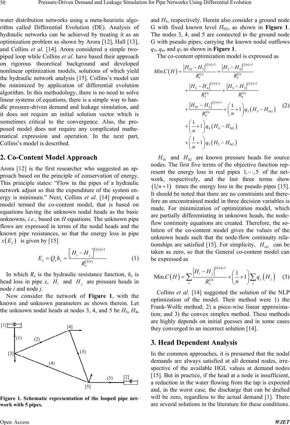

Pressure-Driven Demand and Leakage Simulation for Pipe Networks Using Differential Evolution

water distribution networks using a meta-heuristic algo-

rithm called Differential Evolution (DE). Analysis of

hydraulic networks can be achieved by treating it as an

optimization problem as shown by Arora [12], Hall [13],

and Collins et al. [14]. Arora considered a simple two-

piped loop while Collins et al. have based their approach

on rigorous theoretical background and developed

nonlinear optimization models, solutions of which yield

the hydraulic network analysis [15]. Collins’s model can

be minimized by application of differential evolution

algorithm. In this methodology, there is no need to solve

linear systems of equations, there is a simple way to han-

dle pressure-driven demand and leakage simulation, and

it does not require an initial solution vector which is

sometimes critical to the convergence. Also, the pro-

posed model does not require any complicated mathe-

matical expression and operation. In the next part,

Collins’s model is described.

2. Co-Content Model Approach

Arora [12] is the first researcher who suggested an ap-

proach based on the principle of conservation of energy.

This principle states: “Flow in the pipes of a hydraulic

network adjust so that the expenditure of the system en-

ergy is minimum.” Next, Collins et al. [14] proposed a

model termed the co-content model, that is based on

equations having the unknown nodal heads as the basic

unknowns, i.e., based on H equations. The unknown pipe

flows are expressed in terms of the nodal heads and the

known pipe resistances, so that the energy loss in pipe



E is given by [15]



xxx n

EQh R









 (1)

In which Rx is the hydraulic resistance function, hx is

head loss in pipe x, i

and are pressure heads in

node i and node j.

Now consider the network of Figure 1, with the

known and unknown parameters as shown therein. Let

the unknown nodal heads at nodes 3, 4, and 5 be H3, H4,

[1]

(1) (2)

[3]

[4]

(3)

(4)

[5]

(5) [2]

Figure 1. Schematic representation of the looped pipe net-

work with 5 pipes.

and H5, respectively. Herein also consider a ground node

G with fixed known level H0G, as shown in Figure 1.

The nodes 3, 4, and 5 are connected to the ground node

G with pseudo pipes, carrying the known nodal outflows

q3, q4, and q5 as shown in Figure 1.

The co-content optimization model is expressed as











 



11 11

01 334

11 11

54 35

02 5

33 0

44 0

550

HH HH

Min CHRR

HH HH

HH qH H

qH H

qHH























 







 







(2)

and 02

are known pressure heads for source

nodes. The first five terms of the objective function rep-

resent the energy loss in real pipes 1, of the net-

work, respectively, and the last three terms show

, 5





11n



times the energy loss in the pseudo pipes [15].

It should be noted that there are no constraints and there-

fore an unconstrained model in three decision variables is

made. For minimization of optimization model, which

are partially differentiating in unknown heads, the node-

flow continuity equations are created. Therefore, the so-

lution of the co-content model gives the values of the

unknown heads such that the node-flow continuity rela-

tionships are satisfied [15]. For simplicity, oG

can be

taken as zero, so that the General co-content model can

be expressed as









Min. 1



CHq H













(3)

Collins et al. [14] suggested the solution of the NLP

optimization of the model. Their method were 1) the

Frank-Wolfe method; 2) a piece-wise linear approxima-

tion; and 3) the convex simplex method. These methods

are highly depends on initial guesses and in some cases

they converged to an incorrect solution [14].

3. Head Dependent Analysis

In the common approaches, it is presumed that the nodal

demands are always satisfied at all demand nodes, irre-

spective of the available HGL values at demand nodes

[15]. But in practice, if the head at a node is insufficient,

a reduction in the water flowing from the tap is expected

and, in the worst case, the discharge that can be drafted

will be zero, regardless to the actual demand [1]. There

are several solutions in the literature for these conditions.

Open Access WJET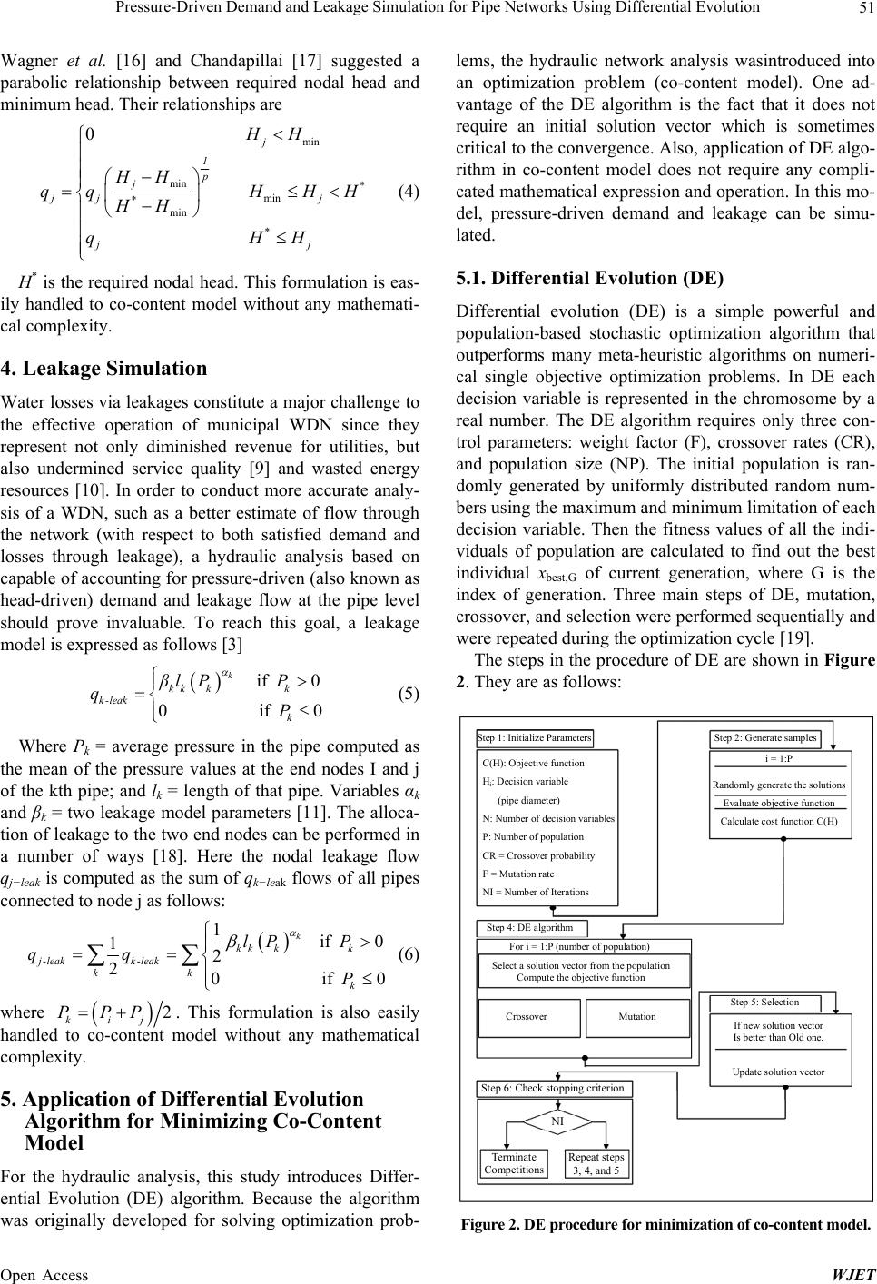

Pressure-Driven Demand and Leakage Simulation for Pipe Networks Using Differential Evolution 51

Wagner et al. [16] and Chandapillai [17] suggested a

parabolic relationship between required nodal head and

minimum head. Their relationships are

min

jj j

qqH HH

qHH















 















(4)

H* is the required nodal head. This formulation is eas-

ily handled to co-content model without any mathemati-

cal complexity.

4. Leakage Simulation

Water losses via leakages constitute a major challenge to

the effective operation of municipal WDN since they

represent not only diminished revenue for utilities, but

also undermined service quality [9] and wasted energy

resources [10]. In order to conduct more accurate analy-

sis of a WDN, such as a better estimate of flow through

the network (with respect to both satisfied demand and

losses through leakage), a hydraulic analysis based on

capable of accounting for pressure-driven (also known as

head-driven) demand and leakage flow at the pipe level

should prove invaluable. To reach this goal, a leakage

model is expressed as follows [3]



if 0

0if

kk kk

k-leak

βlPP













(5)

Where Pk = average pressure in the pipe computed as

the mean of the pressure values at the end nodes I and j

of the kth pipe; and lk = length of that pipe. Variables αk

and βk = two leakage model parameters [11]. The alloca-

tion of leakage to the two end nodes can be performed in

a number of ways [18]. Here the nodal leakage flow

qj−leak is computed as the sum of qk−leak flows of all pipes

connected to node j as follows:



1if 0

20if

kk kk

jleakkleak

lP P













0





 (6)

where





kij

PPP . This formulation is also easily

handled to co-content model without any mathematical

complexity.

5. Application of Differential Evolution

Algorithm for Minimizing Co-Content

Model

For the hydraulic analysis, this study introduces Differ-

ential Evolution (DE) algorithm. Because the algorithm

was originally developed for solving optimization prob-

lems, the hydraulic network analysis wasintroduced into

an optimization problem (co-content model). One ad-

vantage of the DE algorithm is the fact that it does not

require an initial solution vector which is sometimes

critical to the convergence. Also, application of DE algo-

rithm in co-content model does not require any compli-

cated mathematical expression and operation. In this mo-

del, pressure-driven demand and leakage can be simu-

lated.

5.1. Differential Evolution (DE)

Differential evolution (DE) is a simple powerful and

population-based stochastic optimization algorithm that

outperforms many meta-heuristic algorithms on numeri-

cal single objective optimization problems. In DE each

decision variable is represented in the chromosome by a

real number. The DE algorithm requires only three con-

trol parameters: weight factor (F), crossover rates (CR),

and population size (NP). The initial population is ran-

domly generated by uniformly distributed random num-

bers using the maximum and minimum limitation of each

decision variable. Then the fitness values of all the indi-

viduals of population are calculated to find out the best

individual xbest,G of current generation, where G is the

index of generation. Three main steps of DE, mutation,

crossover, and selection were performed sequentially and

were repeated during the optimization cycle [19].

The steps in the procedure of DE are shown in Figure

2. They are as follows:

Terminate

Competitions

Repeat steps

3, 4, and 5

Step 6: Check stopping criterion

Step 1: Initialize Parameters Step 2: Generate samples

C(H): Objective function

Hi: Decision variable

(pipe diameter)

: Number of decision variables

P: Number of population

CR = Crossover probability

F = Mutation rate

I = Number of Iterations

i = 1:P

Randomly generate the solutions

Evaluate objective function

Calculate cost function C(H)

Step 4: DE algorithm

For i = 1:P (number of population)

Select a solution vector from the population

Compute the objective function

Crossover Mutation

Step 5: Selection

If new solution vector

Is better than Old one.

Update solution vector

Figure 2. DE procedure for minimization of co-content model.

Open Access WJET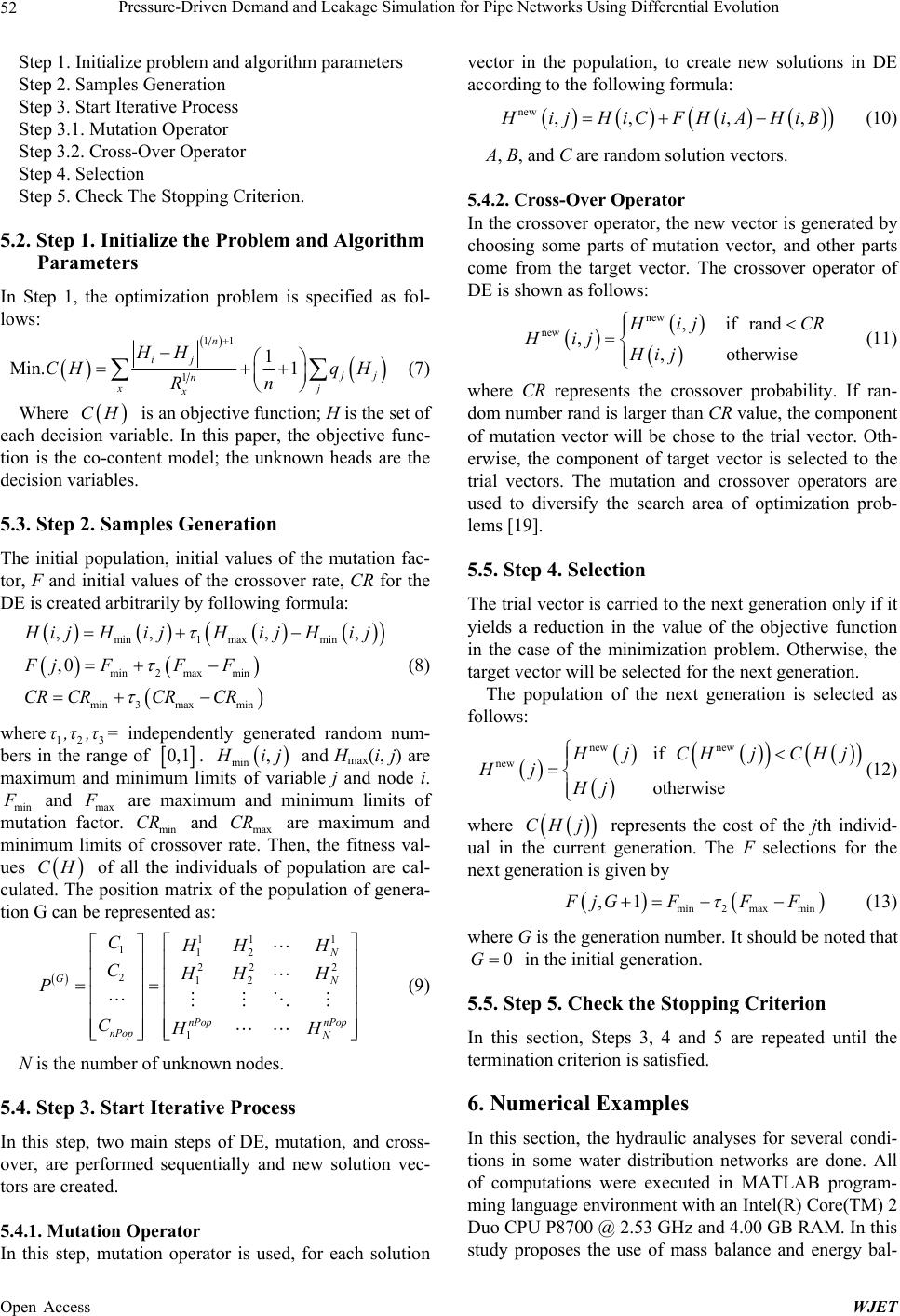

Pressure-Driven Demand and Leakage Simulation for Pipe Networks Using Differential Evolution

Step 1. Initialize problem and algorithm parameters

Step 2. Samples Generation

Step 3. Start Iterative Process

Step 3.1. Mutation Operator

Step 3.2. Cross-Over Operator

Step 4. Selection

Step 5. Check The Stopping Criterion.

5.2. Step 1. Initialize the Problem and Algorithm

Parameters

In Step 1, the optimization problem is specified as fol-

lows:









Min. 1



CHq H













(7)

Where





CH is an objective function; H is the set of

each decision variable. In this paper, the objective func-

tion is the co-content model; the unknown heads are the

decision variables.

5.3. Step 2. Samples Generation

The initial population, initial values of the mutation fac-

tor, F and initial values of the crossover rate, CR for the

DE is created arbitrarily by following formula:

 





min1maxmin

min2 maxmin

min 3maxmin

,, ,



ijHij HijHij

FjFF F

CR CRCRCR



 

(8)

where 123

= independently generated random num-

bers in the range of

τ,τ,τ





0,1 .





min ,

ij and Hmax(i, j) are

maximum and minimum limits of variable j and node i.

min

and max

are maximum and minimum limits of

mutation factor. min and max are maximum and

minimum limits of crossover rate. Then, the fitness val-

ues of all the individuals of population are cal-

culated. The position matrix of the population of genera-

tion G can be represented as:

CR CR



11 1

112

22 2

212

nPop nPop

nPop N

CHH H

CHHH

CHH





































(9)

N is the number of unknown nodes.

5.4. Step 3. Start Iterative Process

In this step, two main steps of DE, mutation, and cross-

over, are performed sequentially and new solution vec-

tors are created.

5.4.1. Mutation Operator

In this step, mutation operator is used, for each solution

vector in the population, to create new solutions in DE

according to the following formula:











new ,, ,,



ijHiCFHiA HiB (10)

A, B, and C are random solution vectors.

5.4.2. Cross-Over Operator

In the crossover operator, the new vector is generated by

choosing some parts of mutation vector, and other parts

come from the target vector. The crossover operator of

DE is shown as follows:









new

new ,ifrand

,,otherwise

ij CR

Hij Hij











(11)

where CR represents the crossover probability. If ran-

dom number rand is larger than CR value, the component

of mutation vector will be chose to the trial vector. Oth-

erwise, the component of target vector is selected to the

trial vectors. The mutation and crossover operators are

used to diversify the search area of optimization prob-

lems [19].

5.5. Step 4. Selection

The trial vector is carried to the next generation only if it

yields a reduction in the value of the objective function

in the case of the minimization problem. Otherwise, the

target vector will be selected for the next generation.

The population of the next generation is selected as

follows:

  



new new

new if

otherwise

jCHjCHj











(12)

where









CH j represents the cost of the jth individ-

ual in the current generation. The F selections for the

next generation is given by









min2maxmin

,1FjGFF F



  (13)

where G is the generation number. It should be noted that



in the initial generation.

5.5. Step 5. Check the Stopping Criterion

In this section, Steps 3, 4 and 5 are repeated until the

termination criterion is satisfied.

6. Numerical Examples

In this section, the hydraulic analyses for several condi-

tions in some water distribution networks are done. All

of computations were executed in MATLAB program-

ming language environment with an Intel(R) Core(TM) 2

Duo CPU P8700 @ 2.53 GHz and 4.00 GB RAM. In this

study proposes the use of mass balance and energy bal-

Open Access WJET

Pressure-Driven Demand and Leakage Simulation for Pipe Networks Using Differential Evolution 53

ance in the network for demonstrating the effectiveness

of DE in comparison with other methods.

The average of mass and energy balance is shown by δ

and is calculated by following formula:



connectedto

through

mean ,

2, ,

abs q























(14)

In all numerical examples ,

min max

min and max . To check the performance

of the DE for the minimization of co-content model, ten

optimization runs were performed using different random

initial solutions in all examples.

0.2CR CR

0.2F0.8F

6.1. Numerical Example 1

In order to demonstrate the advantages of the proposed

model in pressure-driven demand condition, the simpli-

fied water distribution network shown in Figure 3, was

used. For the sake of simplicity, the same Hazen-Wil-

liams roughness coefficient C = 130 was assumed for all

the 14 pipes of identical length of 1000 m, while no mi-

nor losses have been added. The following diameters

have been used in the example: 500 mm (P-2); 400 mm

(P-1); 300 mm (P-4, P-7); 250 mm (P-10); 200 mm (P-3,

P-5, P-6, P-13); 150 mm (P-8, P-9, P-11, P-12, P-14).

The nodal demands are q2 = 1, q3 = 1, q4 = 2, q5 = 15, q6

= 15, q7 = 10, q8 = 5 (m3/min). Without loss of general-

Reservoir

1 2

4 8

5 6 7

10 11 12 13

7 8

Figure 3. Schematic representation of the looped pipe net-

work used in the numerical example 1.

ity, in this example, the minimum head requirement *

has been assumed equal to the ground elevation Zi [1]. So

the relationship between required nodal head and mini-

mum head is:

qqZ H













(15)

Todini [1] proposed a three steps approach for solving

this network and its solution is reported in the 4th col-

umn of Table 1. In proposed methodology, pressure-

driven model can be applied in hydraulic analysis with-

out any mathematical formulation. In this situation, an

if-then rule is added to co-content model and optimiza-

tion process is conducted. The DE technique is applied to

solve this problem in three cases. DE model parameters

selected are as follows: number of decision variables = 7;

number of population for case 1 = 10, case 2 = 20, case 3

= 20; number of iteration for case 1 = 1000, case 2 =

1000 and case 3 = 5000. The bound variables were set

between 50 and 140. The best, worst and average solu-

tions of DE algorithm in three cases are shown in Table

2. This table compares the average of mass and energy

balance of the three cases with those obtained using To-

dini algorithm. As it can be seen in Table 2, DE found

the optimal solution more accurately than Todini method

in all cases. Results of the best performance of DE and

convergence history are reported in Table 1 and Figure

4, respectively.

As you can see in the Figure 4, after about 400 itera-

tions the parameter δ becomes convergent and then it

doesn’t change. The minimum value of δ calculated by

DE algorithm is 2.07E-02, while the value obtained for

this parameter, by the method introduced by Todini

equals to 2.76E-02. Values of δ at each node are com-

pared in the seventh and eighth columns of Table 1, us-

ing the two proposed methods and the method of Todini.

0100 200300 400500 600 700800 9001000

-2

-1

Number of It erat ion

Average o

Mass and E nergy Bal anc e

Figure 4. Convergence history of numerical example 1.

Open Access WJET

Pressure-Driven Demand and Leakage Simulation for Pipe Networks Using Differential Evolution

Open Access WJET

Table 1. Head and parameter δ in numerical example 1.

DE 3 steps DE 3 steps DE 3 steps

Node Z(m)

H(m) H(m) [2] H-Z H-Z [1] δ δ [1]

1 140 140 140 0 0 0 0

2 80 129.304 130.07 49.304 50.07 7.93e-10 0.0003

3 90 132.288 132.76 42.288 42.76 7.24e-09 0.004

4 70 109.587 110.96 39.587 40.96 5.56e-10 0.0021

5 80 80.000 88.54 0.000 8.54 0.0576 0.034

6 90 90.000 91.45 0.000 1.45 0.0069 0.0173

7 90 90.000 90.00 0.000 0.00 0.0803 0.106

8 100 88.922 90.43 −11.078 −9.57 2.54e-09 0.0439

Table 2. Average of mass and energy balance for numerical example 1.

Mass and Energy Balance (δ)

best worst mean std

Number of population 10

Number of iteration 1000

2.07E-02 9.01E-02 4.14E-02 2.37E-02

Number of population 20

Number of iteration 1000

2.07E-02 2.08E-02 2.07E-02 3.38E-05

Number of population 20

Number of iteration 5000

2.07E-02 2.07E-02 2.07E-02 6.20E-06

Three Steps Approach [1] Maximum Accuracy 2.76E-02

As you can see at all the nodes, in calculating the mini-

mum value of δ, the proposed method works better than

the Todini method.

6.2. Numerical Example 2

The second considered network is a real planned network

designed for an industrial area in Apulian town (Southern

Italy). The network layout is shown in Figure 5 and the

corresponding data are provided in Table 3. With respect

to the leakages, they have been assumed as pressure-

driven (see Equation (5)) since they are implemented in

the pressure-driven network simulation model as above

described [11]. The parameter β = 1.0632 × 10 − 7 and α

= 1.2, as reported in Giustolisi et al. [11] for this network.

Giustolisi et al. [11] proposed a hydraulic simulation

model, which fully integrates a classic hydraulic simula-

tion algorithm, such as that of Todini and Pilati [20]

found in EPANET 2, with a pressure-driven model that

entails a more realistic representation of leakage. They

applied their model in this network and results are dem-

Figure 5. Schematic representation of the looped pipe net-

work used in the numerical example 4.

onstrated in Table 4. The DE technique is applied to

solve this problem and DE model parameters selected are

as follows: number of decision variables = 23; number of

population for all case 1 = 50, case 2 = 50, case 3 = 20,

Pressure-Driven Demand and Leakage Simulation for Pipe Networks Using Differential Evolution 55

Table 3. Hydraulic data relevant to the numerical example

Pipe L (m) D (mm) Pipe L (m)D (mm) Pipe L (m)D (mm)

1 348.5 327 12 428.4184 23 165.5 100

2 955.7 290 13 419 100 24 252.1100

3 483 100 14 1023.1100 25 331.5100

4 400.7 290 15 455.1164 26 500204

5 791.9 100 16 182.6290 27 579.9 164

6 404.4 368 17 221.3290 28 842.8 100

7 390.6 327 18 583.9164 29 792.6 100

8 482.3 100 19 452 229 30 846.3184

9 934.4 100 20 794.7100 31 164258

10 431.3 184 21 717.7100 32 427.9100

11 513.1 100 22 655.6258 33 379.2100

34 158.2368

case 4 = 20 and case 5 = 50; number of iteration for case

1 = 500, case 2 = 1000, case 3 = 10,000, case 4 = 5000

and case 4 = 2500. In proposed method, there is no need

to change mathematical formulation for hydraulic analy-

sis. An if-then rule is added to co-content model and op-

timization process is done easily. In this example, the

bound variables were set between 0 and 36.4.

Table 5 compares different cases of algorithm DE for

minimization of model. The best result is related to the

case in which the number of population is equal to 50

and the number of iterations equal to 2500. After per-

forming 10 different runs, the best value of δ is obtained

equal to 0.0026, while the best result is obtained equal to

0.0181 in Giustolis method. The results of two men-

tioned methods are compared in the fifth and sixth col-

umns of Table 4. In this table, the best result is shown in

bold, and it is considered the method DE has calculated

the best value of δ at 17 nodes and Gistulishi method has

calculated it at 5 nodes. The convergence process of al-

gorithm DE has been shown in two forms in Figures 6

and 7. The absolute value of δ is calculated for each it-

eration in Figure 6 and the amount of objective function

C(H) is calculated for each iteration in Figure 7. The

algorithm becomes convergent after 2500 iterations.

6.3. Numerical Example 3

Figure 8 shows the network from Mallick et al. [21].

The network consists of 2 reservoirs, 13 nodes and 21

pipes. The detailed properties are shown in Tables 6 and

7. It is supposed that the desired pressure for each node

(H*) is 30 m, and the minimum pressure (Hmin) is 10 m

[22]. The pipe leakage coefficients are β = 5 × 10 − 7 and

Table 4. Head and parameter δ in numerical example 2.

Node H

number

q (l/s)

(m) [1]

H (m) δ [11] δ

1 10.86326.9 33.29 0.1547426

−0.0046

2 17.03424.81 31.83 0.02131049

−0.00648

3 14.94721.3 27.39 −0.0477137 −0.00498

4 14.2817.22 25.34 −0.0220368 −0.00504

5 10.13323.54 30.89 −0.0261836 −0.00378

6 15.3520.1 29.02 0.04038949

−0.00517

7 9.11418.91 27.94 −0.0171474 −0.00275

8 10.5117.9 27.34

−0.0022701 −0.00351

9 12.18217.85 26.35

0.0029365 −0.00378

10 14.57912.66 23.24 −0.008277 −0.0043

11 9.00716.23 25.95 0.03155407

−0.00258

12 7.57510.12 22.05 −0.0027315 −0.00213

Node H

number

q (l/s)

(m) [11]

H (m) δ [11] δ

13 15.210.03 22.45 0.01259978

−0.00418

14 13.5515.41 25.95 0.06347619

−0.00418

15 9.22614 24.17 −0.0091379 −0.00287

16 11.214.36 24.05 −0.0070886 −0.00357

17 11.46915.3 25.42

−0.0001028 −0.00354

18 10.81818.83 28.38 0.01188886

−0.00384

19 14.67519.35 28.39

−5.43E-05 −0.00505

20 13.31810.01 23.79 −0.0377624 −0.00398

21 14.63111.48 22.35

0.00274996 −0.00411

22 12.01214 25.46 0.00390141

−0.0036

23 10.32610.45 20.11 −0.0085767 −0.00296

24 36.45 36.45

α = 1.18, for this network. The DE technique is applied

to solve this problem and DE model parameters selected

are as follows: number of decision variables = 13; num-

ber of population for all cases = 20; number of iteration

for case 1 = 1000, case 2 = 2500, case 3 = 5000 and case

4 = 10,000. The bound variables were set between 0 and

60.96.

In this example, the network has been analyzed ac-

cording to two cases. In the first case, the dependence of

pressure on the demand is not included, but in the latter

case, the analysis is performed by taking into account the

dependence of pressure on the demand. Table 8 shows

Open Access WJET

Pressure-Driven Demand and Leakage Simulation for Pipe Networks Using Differential Evolution

05001000 1500 2000 2500

10-3

10-2

10-1

100

Number of Iterat i on

Average of M ass and E nergy Bal ance

Figure 6. Convergence history of numerical example 2 (case

1).

0500 1000 1500 2000 2500

1.2

1.3

1.4

Number of Iterat i on

Obje ctive Functi on C(H)

Figure 7. Convergence history of numerical example 2 (case

2).

Figure 8. Schematic representation of the looped pipe net-

work used in the numerical example 3.

Table 5. Average of mass and energy balance for numerical

example 2.

Mass and Energy Balance (δ)

best worst mean std

Number of

population 50

Number of

iteration 500

6.00E-03 1.76E-02 1.14E-023.60E-03

Number of

population 50

Number of

iteration 1000

2.60E-03 1.01E-02 5.90E-032.20E-03

Number of

population 20

Number of

iteration 10,000

3.90E-03 4.00E-03 4.00E-034.08E-05

Number of

population 20

Number of

iteration 5000

3.20E-03 3.80E-03 3.60E-031.88E-04

Number of

population 50

Number of

iteration 2500

2.60E-03 5.50E-03 3.00E-035.88E-04

Giustolisi

Algorithm [11]Maximum Accuracy 1.81E-02

Table 6. Pipe characteristics of Sample network from Mal-

lick et al. [21].

Pipe Number L (m) D (mm) C

1 609.6 762 130

2 243.8 762 128

3 1524 609 126

4 1127.76 609 124

5 1188.72 406 122

6 640.08 406 120

7 762 254 118

8 944.88 254 116

9 1676.4 381 114

10 883.92 305 112

11 883.92 305 110

12 1371.6 381 108

13 762 254 106

14 822.96 254 104

15 944.88 305 102

16 579 305 100

17 487.68 203 98

18 457.2 152 96

19 502.92 203 94

20 883.92 203 92

21 944.88 305 90

Open Access WJET

Pressure-Driven Demand and Leakage Simulation for Pipe Networks Using Differential Evolution 57

Table 7. Nodes properties of Sample network from Mallick

et al. [21].

Node Number q (L/S) Elevation (m)

1 0 27.43

2 59 33.53

3 59 28.96

4 178 32

5 59 30.48

6 190 31.39

7 178 29.56

8 91 31.39

9 0 32.61

10 0 34.14

11 30 35.05

12 30 36.58

13 0 33.53

Table 8. Average of mass and energy balance for numerical

example 3.

Mass and Energy Balance (δ)

best worst mean std

Number of

population 20

Number of

iteration 1000

1.90E-031.11E-02 5.30E-032.60E-03

Number of

population 20

Number of

iteration 2500

1.46E-047.03E-04 4.55E-041.72E-04

Number of

population 20

Number of

iteration 5000

1.06E-061.37E-06 5.00E-064.32E-06

Number of

population 20

Number of

iteration 10,000

1.18E-082.90E-08 1.75E-086.29E-09

how the accuracy of parameter δ depends on the iteration

number of convergence in the first case. As it can be seen,

the value of δ reaches the accuracy 1e-2 after 1000 itera-

tions, the accuracy 1e-4 after 2500 iterations, 1e-6 after

5000 iterations and 1e-8 after 10,000 iterations. Figure 9

compares the nodal pressures in the mentioned two cases.

As it can be observed, if the dependence of pressure on

the demand is not included, a negative pressure is made

at the nodes 6, 8, 11 and 12, but all pressures in the sec-

ond case are greater than 5 meters and the minimum

pressure of 10 meters has been partly supplied in most of

the nodes. Figure 10 shows the process of changing the

Figure 9. Simulation results with and without pressure-

driven demand.

01000 20003000 4000 5000 60007000 80009000 10000

10-8

10-7

10-6

10-5

10-4

10-3

10-2

10-1

100

Number of Iterati on

A v erage of Mass and E nergy Bal an c e

Figure 10. Convergence history of numerical example 3.

parameter δ towards the number of iterations.

7. Conclusions

The purpose of this paper has been to introduce a novel

methodology for hydraulic analysis of water distribution

systems under deficient pressure conditions considering

the pressure-driven demand and leakage. The methodol-

ogy is illustrated using three networks with different

layouts.

The overall results indicate that the proposed method

has the capability to handle various pipe networks prob-

lems without changing in model and mathematical for-

mulation. Application of DE to co-content model can

solve pressure-driven demand and leakage simulation

with applying if-then rules in co-content model. The ad-

vantage of the proposed methodology is its flexibility in

employing different formulation and specifying parame-

ters related to pressure-driven demand. Another advan-

tage of this method is that it can be easily developed for

Open Access WJET

Pressure-Driven Demand and Leakage Simulation for Pipe Networks Using Differential Evolution

Open Access WJET

common users to undertake deficient pressure conditions.

REFERENCES

[1] E. Todini, “A More Realistic Approach to the “Extended

Period Simulation” of Water Distribution Networks, Ad-

vances in Water Supply Management,” Taylor & Francis,

Chapter 19, 2003.

[2] F. Martinez, P. Conejos and J. Vercher, “Developing an

Integrated Model for Water Distribution Systems Con-

sidering Both Distributed Leakage and Pressure Depend-

ent Demands,” Proceedings of the 26th Annual ASCE

Water Resources Planning and Management Conference,

Tempe, Arizona, June 1999, pp. 1-14.

[3] G. Germanopoulos, “A Technical Note on the Inclusion

of Pressure Dependent Demand and Leakage Terms in

Water Supply Network Models,” Civil Engineering and

Environmental Systems, Vol. 2, No. 3, 1985, pp. 171-179.

http://dx.doi.org/10.1080/02630258508970401

[4] G. Germanopoulos, P. W. Jowitt and J. P. Lumbers, “As-

sessing the Reliability of Supply and Level of Service for

Water Distribution Systems,” Proceedings of The Institu-

tion of Civil Engineers, Vol. 80, No. 2, 1 April 1986, pp.

413-428.

http://dx.doi.org/10.1680/iicep.1986.741

[5] J. Lumbers, “Re-Thinking Network Analysis for Inter-

mittent Supplies,” Water and Environment, Manager, Vol.

1, No. 3, 1996, p. 6.

[6] L. S. Reddy and K. Elango, “Analysis of Water Distribu-

tion Networks with Head Dependent Outlets,” Civil En-

gineering Systems, Vol. 3, No. 6, 1989, pp. 102-110.

http://dx.doi.org/10.1080/02630258908970550

[7] M. Tabesh, “Implications of the Pressure Dependency of

Outflows on Data Management, Mathematical Modeling

and Reliability Assessment of Water Distribution Sys-

tems,” PhD Thesis, University of Liverpool, Liverpool,

UK, 1998.

[8] T. T. Tanyimboh and M. Tabesh, “Discussion of Com-

parison of Methods for Predicting Deficient-Network

Performance,” Journal of Water Resources Planning and

Management, Vol. 123, No. 6, 1997, pp. 369-370.

[9] J. Almandoz, E. M. Cabrera, F. Arregui, E. Jr. Cabrera

and R. Cobacho, “Leakage Assessment through Water

Distribution Network Simulation,” Journal of Water Re-

sources Planning and Management, Vol. 131, No. 6,

2005, pp. 458-466.

http://dx.doi.org/10.1061/(ASCE)0733-9496(2005)131:6(

458)

[10] A. F. Colombo and B. W. Karney, “Energy and Costs of

Leaky Pipes: Toward a Comprehensive Picture,” Journal

of Water Resources Planning and Management, Vol. 128,

No. 6, 2002, pp. 441-450.

[11] O. Giustolisi, D. Savic and Z. Kapelan, “Pressure-Driven

Demand and Leakage Simulation for Water Distribution

networks,” Journal of Hydraulic Engineering, Vol. 134,

No. 5, 2008, pp. 626-635.

http://dx.doi.org/10.1061/(ASCE)0733-9429(2008)134:5(

626)

[12] M. L. Arora, “Flow Split In Closed Loops Expending

Least Energy,” Journal of the Hydraulics Division, Vol.

102, No. 3, 1976, pp. 455-458.

[13] M. A. Hall, “Hydraulic Network Analysis Using (Gener-

alized) Geometric Programming,” Networks, Vol. 6, No. ,

6, 1976, pp. 105-130.

http://dx.doi.org/10.1002/net.3230060204

[14] M. Collins, L. Cooper, R. Helgason, J. Kenningston and

L. LeBlanc, “Solving the Pipe Network Analysis Problem

Using Optimization Techniques,” Management Science,

Vol. 24, No. 7, 1978, pp. 747-760.

http://dx.doi.org/10.1287/mnsc.24.7.747

[15] P. R. Bhave and R. Gupta, “Analysis of Water Distribu-

tion Networks,” Alpha Science International, Technology

& Engineering, University of Michigan, Michigan, 2006.

[16] J. Wagner, U. Shamir and D. Marks, “Water Distribution

Reliability: Analytical Methods,” Journal of the Water

Resources Planning and Management, Vol. 114, No. 3,

1988, pp. 253-275.

http://dx.doi.org/10.1061/(ASCE)0733-9496(1988)114:3(

253)

[17] J. Chandapillai, “Realistic Simulation of Water Distribu-

tion System,” Journal of Transportation Engineering,

Vol. 117, No. 2, 1991, pp. 258-263.

http://dx.doi.org/10.1061/(ASCE)0733-947X(1991)117:2

(258)

[18] L. Ainola, T. Koppel, T. Tiiter and A. Vassiljev, “Water

Network Model Calibration Based on Grouping Pipes

with Similar Leakage and Roughness Estimates,” Pro-

ceedings of the Joint Conference on Water Resource En-

gineering and Water Resource Planning and Manage-

ment, Minneapolis, 2000, pp. 104-197.

[19] W. Chun-Yin and T. Ko-Ying, “Topology Optimization

of Structure Using Differential Evolution,” Journal of

Systemics, Cybernetics and Informatics, Vol. 42, No. 6,

2008, pp. 46-51.

[20] E. Todini and S. Pilati, “A Gradient Algorithm for the

Analysis of Pipe Networks. Computer Applications in

Water Supply. 1 (System Analysis and Simulation),” John

Wiley & Sons, London, 1988, pp. 1-20.

[21] K. N. Mallick, I. Ahmed, K. S. Tickle and K. E. Lansey,

“Determining Pipe Groupings For Water Distribution

Networks,” Journal of Water Resources Planning and

Management, Vol. 128, No. 2, 2002, pp. 130-139.

http://dx.doi.org/10.1061/(ASCE)0733-9496(2002)128:2(

130)

[22] L. Jun and Y. Guoping, “Iterative Methodology of Pres-

sure-Dependent Demand Based on EPANET for Pres-

sure-Deficient Water Distribution Analysis,” Journal of

Water Resources Planning Management, Vol. 139, No. 1,

2013, pp. 34-44.

http://dx.doi.org/10.1061/(ASCE)WR.1943-5452.000022