Feature Extraction by Multi-Scale Principal Component Analysis and Classification in Spectral Domain

doi:10.4236/eng.2013.510B056

Paper Menu >>

Journal Menu >>

Engineering, 2013, 5, 268-271

http://dx.doi.org/10.4236/eng.2013.510B056 Published Online October 2013 (http://www.scirp.org/journal/eng)

Feature Extraction by Multi-Scale Principal Component

Analysis and Classification in Spectral Domain

Shengkun Xie1*, Anna T. Lawnizak2, Pietro Lio’3, Sridhar Krishnan4

1Global Management Studies, Ryerson University, Toronto, Canada

2Department of Mathematics and Statistics, University of Guelph, Guelph, Canada

3Computer Laboratory, University of Cambridge, Cambridge, UK

4Electrical and Computer Engineering, Ryerson University, Toronto, Canada

Email: *[email protected]

Received June 2013

ABSTRACT

Feature extraction of signals plays an important role in classification problems because of data dimension reduction

property and potential improvement of a classification accuracy rate. Principal component analysis (PCA), wavelets

transform or Fourier transform methods are often used for feature extraction. In this paper, we propose a multi-scale

PCA, which combines discrete wavelet transform, and PCA for feature extraction of signals in both the spatial and

temporal domains. Our study shows that the multi-scale PCA combined with the proposed new classification methods

leads to high classification accuracy for the considered signals.

Keywords: Multi-Scale Principal Component Analysis; Discrete Wavelet Transform; Feature Extra ction ; S ign a l

Classification; Empirical Classification

1. Introduction

The performance of a method used to recover the deter-

ministic pattern is often impacted by stochastic correla-

tions among noises of signals. As a common multivariate

statistical method, the principal component analysis

(PCA) [1] is often used for data dimension reduction and

feature extraction of signals. The data features can be

extracted by mapping signals onto a feature subspace that

is spanned by only the first few principal components.

However, the classical PCA may not perform well when

it is applied to temporally correlated data or non-statio-

nary data. When PCA is applied to these types of data,

two following common problems are encountered. The

first one is that PCA of measurements of stochastic

processes is a single scale modeling approach, which

means that local measurements do not vary with diff erent

underlying frequencies. Data from complex systems are

often multi-scale and non-stationary in nature [2], there-

fore the conventional PCA often is not suitable for ana-

lyzing these typesof data. The second problem is that

most of the data coming from complex systems are often

temporally correlated.

Since PCA is based on the analysis of the data va-

riance-covariance matrix, to avoid the potential undesir-

able effects on the outcomes of PCA caused by autocor-

relation of the data, one may improve the data analysis

by applying instead PCA in wavelet domain of the data,

i.e. to the transformed data obtained by taking discrete

wavelet transform (DWT), or wavelet packet transform,

or stationary wavelet transform of the original data. The

reason is that in wavelet domain the data have good de-

correlation and localization properties [3]. The encoun-

tered problems of the conventional PCA when applying

to auto-correlated or non-stationary data can be resolved

by combining wavelet transforms with PCA because the

wavelet coefficients of the data at each wavelet scale are

approximately stationary and temporally uncorrelated

([4,5]). Additionally, due to the fact that in wavelet do-

main the significant features of the data can be extracted

by a set of large values of wavelet and scaling coeffi-

cients and the fact that PCA can explain the large varia-

tions through few principal components, the combination

of DWT with PCA can extract spatial and temporal data

features simultaneously. In this paper, we illustrate the

usefulness of DWT and PCA to the classification prob-

lem of a set of EEG data. We propose two methods,

namely confidence interval classification and empirical

classification, to classify the extracted features in the

spectral domain.

2. Methods

2.1. Multi-Scale Principal Component Analysis

In the multi-scale PCA approach, first, signals are orga-

Corresponding author.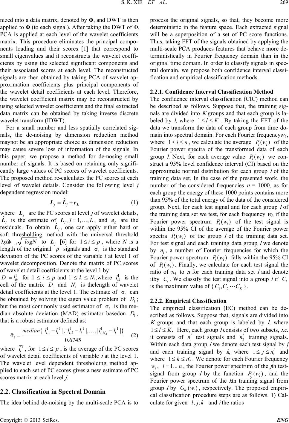

S. K. XIE ET AL.

269

nized into a data matrix, denoted by Φ, and DWT is th en

applied to Φ (to each signal). After taking the DWT of Φ,

PCA is applied at each level of the wavelet coefficients

matrix. This procedure eliminates the principal compo-

nents loading and their scores [1] that correspond to

small eigenvalues and it reconstructs the wavelet coeffi-

cients by using the selected significant components and

their associated scores at each level. The reconstructed

signals are then obtained by taking PCA of wavelet ap-

proximation coefficients plus principal components of

the wavelet detail coefficients at each level. Therefore,

the wavelet coefficient matrix may be reconstructed by

using selected wavelet coefficients and the final extracted

data matrix can be obtained by taking inverse discrete

wavelet transform (IDWT).

For a small number and less spatially correlated sig-

nals, the de-noising by dimension reduction method

maynot be an appropriate choice as dimension reduction

may cause severe loss of information of the signals. In

this paper, we propose a method for de-nosing small

number of signals. It is based on retaining only signifi-

cantly large values of PC scores of wavelet coefficients.

The propos ed method re-calculates the PC scores at each

level of wavelet details. Consider the following level

dependent regre s s i on model:

= +

L Le

(1)

where

are the PC scores at level

of wav elet details,

is the estimate of

,1, ,

jL= …L

, and

are the

residuals. To obtain

, one can apply either hard or

soft thresholding method with the universal threshold

λσ2

logN=

[6] for

1ip≤≤

, where N is a

length of the original

signals and

is the standard

deviation of the PC scores of the variable i at level 1 of

wavelet decomposition. Denote the matrix of PC scores

of wavelet detail coefficients at the level 1 by

1ik

Dl=

for 1 ≤ i ≤ p and 1 ≤ k ≤ N1,where

is the

cell of the matrix

and

is thelength of wavelet

detail coefficients at the lev el 1. The estimate of

can

be obtained by solving the eigen value problem of

;

but the most commonly used estimator of

is the me-

dian absolute deviation (MAD) estimator basedon

that is a robust estimator defined as:

1 11111

,1 ,2,

{||,||, ,||}

σ0.6745

iiiiiN i

median llllll−−… −

(2)

where

, for

1ip≤≤

, is the average of the PC scores

of wavelet detail coefficients of variable

at the level 1.

The wavelet level dependent thresholding method ap-

plied to each set of PC scores gives a new estimate of PC

scores matrix at each level

2.2. Classification in Spectral Domain

The idea behind de-noising by the multi-scale PCA is to

process the original signals, so that, they become more

deterministic in the feature space. Each extracted signal

will be a superposition of a set of PC score functions.

Thus, taking FFT of the sign als obtained by applying the

mul ti -scale PCA produces features that behave more de-

terministically in Fourier frequency domain than in the

original time domain. In order to classify signals in spec-

tral domain, we propose both confidence interval classi-

fication and empirical classification methods.

2.2.1. Confidence Interval Classification Method

The confidence interval classification (CIC) method can

be described as follows. Suppose that, the training sig-

nals are divided into

groups and that each group is la-

beled by

, where

1lK≤≤

. By taking the FFT of the

data we transform the data of each group from time do-

main into spectral domain. For each Fourier frequency,

where

1in≤≤

, we calculate the average

()

of the

Fourier power spectra of the transformed data of each

group

. Next, for each average value

()

we con-

struct a 95% level confidence interval (CI) based on the

approximate normal distribution for each group

of the

training data set. In the case of the presented work, the

number of the considered frequencies

= 1000, as for

each group the energy of these 1000 points contains more

than 95% of the total energy of the data of the considered

group. Next, for each test signal and for each group

the training data set we test, for each frequency

, if the

Fourier power spectrum

()

of the test signal is

within the 95% CI of the average of the Fourier power

spectra

()

of the group

of the training data set.

For test signal and each training data group

we denote

, a number of Fourier frequencies for which the

Fourier power spectrum

()

falls within the 95% CI

()

. Finally, we calculate for each test signal the

ratio of  to

for each training data set

and denote

itby

. We classify the test signal into a group

is the maximum value of {

CC C

2.2.2. Empirical Classification

The empirical classification (EC) method can be de-

scribed as follows. Suppose that, signals are divided into

groups and that each group is labeled by

, where

1.lK≤≤

Here, each group

consists of two subsets,

i.e

it consists of

test signals and

training signals.

Within each data group

we denote each test signal by

and each training signal by

where 1

≤≤ and

where

kn≤≤

. We denote for each Fourier frequ ency

1... in=

, the Fourier power spectrum of the

th test-

signal from group

by the function

()

lj i

, and the

Fourier power spectrum of the

th training signal from

group

()

lk i

, respectively. The proposed empiri-

cal classification procedure steps are as follows. 1) Cal-

culate f or given

,,l jk

and

the ratios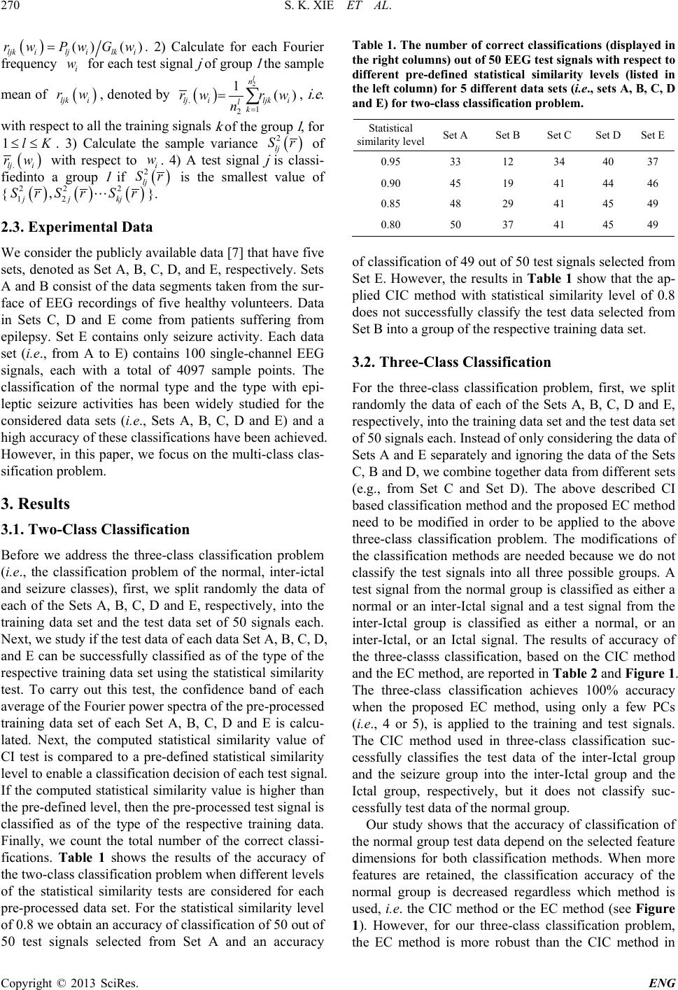

S. K. XIE ET AL.

270

( )

() ()

ljkilj ilki

rwPwG w=

. 2) Calculate for each Fourier

frequency

for each test signal

of group

the sample

mean of

( )

ljk i

, denoted by

( )

1()

ljiljk i

w rw

∑

i.e

with respect to all the training signals

of the group

, for

1lK≤≤

. 3) Calculate the sample variance

( )

S r

( )

.lj i

r w

with respect to

. 4) A test signal

is classi-

fiedinto a group

( )

S r

is the smallest value of

{

( )( )()

22 2

j jkj

SS Srr r

2.3. Experimental Data

We consider the publicly available data [ 7] that h ave five

sets, denoted as Set A, B, C, D, and E, respectively. Sets

A and B consist of the data segments taken from the sur-

face of EEG recordings of five healthy volunteers. Data

in Sets C, D and E come from patients suffering from

epilepsy. Set E contains only seizure activity. Each data

set (i.e., from A to E) contains 100 single-channel EEG

signals, each with a total of 4097 sample points. The

classification of the normal type and the type with epi-

leptic seizure activities has been widely studied for the

considered data sets (i.e., Sets A, B, C, D and E) and a

high accuracy of these classifications have been achieved.

However, in this paper, we focus on the multi-class clas-

sification problem.

3. Results

3.1. Two-Class Classificat ion

Before we address the three-class classification problem

(i.e., the classification problem of the normal, inter-ictal

and seizure classes), first, we split randomly the data of

each of the Sets A, B, C, D and E, respectively, into the

training data set and the test data set of 50 signals each.

Next, we study if the test data of each data Set A, B, C, D,

and E can be successfully classified as of the type of the

respective training data set using the statistical similarity

test. To carry out this test, the confidence band of each

average of the Fourier power sp ectra of the pre-processed

training data set of each Set A, B, C, D and E is calcu-

lated. Next, the computed statistical similarity value of

CI test is compared to a pre-defined statistical similarity

level to enable a classification decision of each test signal.

If the computed statistical similarity value is higher than

the pre-defined level, then the pre-processed test signal is

classified as of the type of the respective training data.

Finally, we count the total number of the correct classi-

fications. Table 1 shows the results of the accuracy of

the two-class classification problem when different levels

of the statistical similarity tests are considered for each

pre-processed data set. For the statistical similarity level

of 0.8 we obtain an accuracy o f classification of 50 out of

50 test signals selected from Set A and an accuracy

Table 1. The number of correct classifications (displayed in

the right columns) out of 50 EEG test signals with respect to

different pre-defined statistical similarity levels (listed in

the left column) for 5 different data sets (i.e., sets A, B, C, D

and E) for two-class classification problem.

Statistical

similarity level Set A Set B Set C Set D Set E

0.95 33 12 34 40 37

0.90 45 19 41 44 46

0.85 48 29 41 45 49

0.80 50 37 41 45 49

of classification of 49 ou t of 50 test signals se lected from

Set E. However, the results in Table 1 show that the ap-

plied CIC method with statistical similarity level of 0.8

does not successfully classify the test data selected from

Set B into a group of the respective training data set.

3.2. Three-Class Classification

For the three-class classification problem, first, we split

randomly the data of each of the Sets A, B, C, D and E,

respectively, into the training data set and the test data set

of 50 signal s each. Inste ad of only co ns ideri ng t he data of

Sets A and E separa tely and ignoring the data of the Sets

C, B and D, we combine together data from different sets

(e.g., from Set C and Set D). The above described CI

based classification method and the proposed EC method

need to be modified in order to be applied to the above

three-class classification problem. The modifications of

the classification methods are needed because we do not

classify the test signals into all three possible groups. A

test signal from the normal group is classified as either a

normal or an inter-Ictal signal and a test signal from the

inter-Ictal group is classified as either a normal, or an

inter-Ictal, or an Ictal signal. The results of accuracy of

the three-classs classification, based on the CIC method

and the EC method, are reported in Table 2 and Figu re 1.

The three-class classification achieves 100% accuracy

when the proposed EC method, using only a few PCs

(i.e., 4 or 5), is applied to the training and test signals.

The CIC method used in three-class classification suc-

cessfully classifies the test data of the inter-Ictal group

and the seizure group into the inter-Ictal group and the

Ictal group, respectively, but it does not classify suc-

cessfully test data of the normal group.

Our study shows that the accuracy of classification of

the normal group test data depend on the selected feature

dimensions for both classification methods. When more

features are retained, the classification accuracy of the

normal group is decreased regardless which method is

used, i.e . the CIC method or the EC method (see Figure

1). However, for our three-class classification problem,

the EC method is more robust than the CIC method in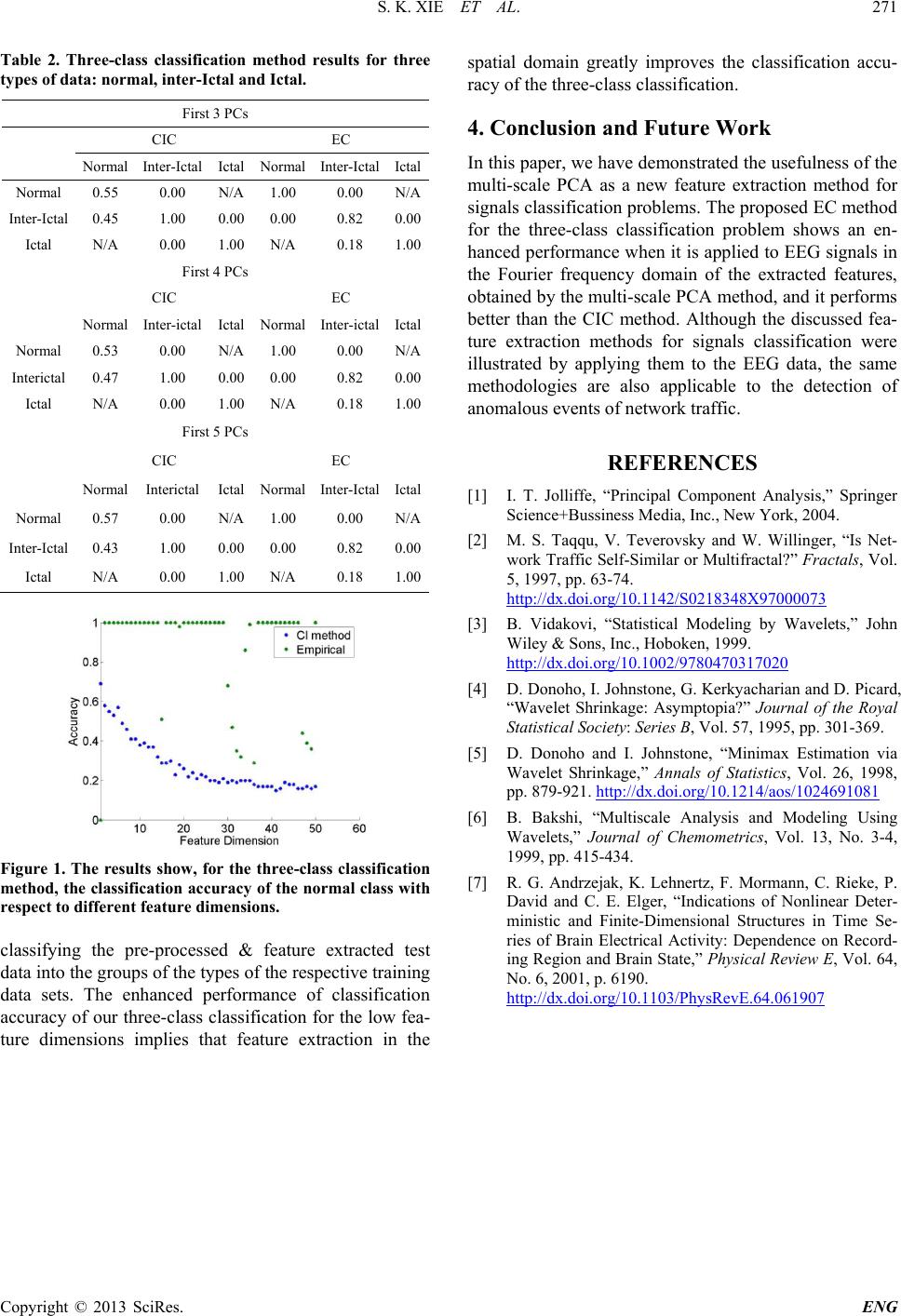

S. K. XIE ET AL.

271

Table 2. Three-class classification method results for three

types of data: normal, inter-Ictal and Ictal.

First 3 PCs

CIC EC

Normal Inter-Ictal Ictal Normal Inter-Ictal Ictal

Normal 0.55 0.00 N/A 1.00 0.00 N/A

Inter-Ictal 0.45 1.00 0.00 0.00 0.82 0.00

Ictal N/A 0.00 1.00 N/A 0.18 1.00

First 4 PCs

CIC EC

Normal Inter-ictal Ictal Normal Inter-ictal Ictal

Normal 0.53 0.00 N/A 1.00 0.00 N/A

Interictal 0.47 1.00 0.00 0.00 0.82 0.00

Ictal N/A 0.00 1.00 N/A 0.18 1.00

First 5 PCs

CIC EC

Normal Interictal Ictal Normal Inter-Ictal Ictal

Normal 0.57 0.00 N/A 1.00 0.00 N/A

Inter-Ictal 0.43 1.00 0.00 0.00 0.82 0.00

Ictal N/A 0.00 1.00 N/A 0.18 1.00

Figure 1. The results show, for the three-class classification

method, the classification accuracy of the normal class with

respect to different feature dimensions.

classifying the pre-processed & feature extracted test

data into the groups of the types of the respective training

data sets. The enhanced performance of classification

accuracy of our three-class classification for the low fea-

ture dimensions implies that feature extraction in the

spatial domain greatly improves the classification accu-

racy of the three -class classification.

4. Conclusion and Future Work

In this paper, we have demonstrated the usefulness of the

mul ti-scale PCA as a new feature extraction method for

signals classification p roblems. The proposed EC method

for the three-class classification problem shows an en-

hanced performance when it is applied to EEG signals in

the Fourier frequency domain of the extracted features,

obtained by the multi-scale PCA method, and it performs

better than the CIC method. Although the discussed fea-

ture extraction methods for signals classification were

illustrated by applying them to the EEG data, the same

methodologies are also applicable to the detection of

anomalous event s of ne t work tra ff i c .

REFERENCES

[1] I. T. Jolliffe, “Principal Component Analysis,” Springer

Science+Bussiness Media, Inc., New York, 2004.

[2] M. S. Taqqu, V. Teverovsky and W. Willinger, “Is Net-

work Traffic Self-Similar or Multifractal?” Fractals, Vol.

5, 1997, pp. 63-74.

http://dx.doi.org/10.1142/S0218348X97000073

[3] B. Vidakovi, “Statistical Modeling by Wavelets,” John

Wiley & Sons, Inc., Hoboken, 1999.

http://dx.doi.org/10.1002/9780470317020

[4] D. Donoho, I. Johnstone, G. Kerkyacharian and D. Picard,

“Wavelet Shrinkage: Asymptopia?” Journal of the Royal

Statistical Society: Series B, Vol. 57, 1995, pp. 301-369.

[5] D. Donoho and I. Johnstone, “Minimax Estimation via

Wavelet Shrinkage,” Annals of Statistics, Vol. 26, 1998,

pp. 879-921. http://dx.doi.org/10.1214/aos/1024691081

[6] B. Bakshi, “Multiscale Analysis and Modeling Using

Wavelets,” Journal of Chemometrics, Vol. 13, No. 3-4,

1999, pp. 415-434.

[7] R. G. Andrzejak, K. Lehnertz, F. Mormann, C. Rieke, P.

David and C. E. Elger, “Indications of Nonlinear Deter-

ministic and Finite-Dimensional Structures in Time Se-

ries of Brain Electrical Activity: Dependence on Record-

ing Region and Brain State,” Physical Review E, Vol. 64,

No. 6, 2001, p. 6190.

http://dx.doi.org/10.1103/PhysRevE.64.061907