Performance Improvement with Combining Multiple Approaches to Diagnosis of Thyroid Cancer

doi:10.4236/eng.2013.510B055

Paper Menu >>

Journal Menu >>

Engineering, 2013, 5, 264-267

http://dx.doi.org/10.4236/eng.2013.510B055 Published Online October 2013 (http://www.scirp.org/journal/eng)

Performance Improvement with Combining

Multiple Approaches to Diagnosis of Thyroid

Cancer

Ahmet Akbaş, Uğur Turhal, Sebahattin Babur, Cafer Avci

Department of Computer Engineering, Yalova University, Yalov a, Turkey

Email: a [email protected], [email protected], [email protected],

[email protected]

Received June 2013

ABSTRACT

There are a lot of diseases that carry death risk when these diseases are infected to human body, if early measures are

not taken. Thyroid cancer is one of them. In USA, number of thyroid cancer cases resulted in death in only 2013 shows

necessity of early fight with this diseas e. This study aims performance improvement in diagn osis of thyroid cancer with

machine learning techniques. Study consists of 3 phases. In the first phase, BayesNet, NaiveBayes, SMO, Ibk and Ran-

dom Forest classifiers have been trained with thyroid cancer train dataset. In the second phase, trained classifiers have

been tested with thyroid cancer test dataset and th e obtained performance results have been compared. In the third and

last phase, approaches named above have been integrated to algorithm AdaboostMI to show difference between of en-

semble classifiers from conventional individual classifiers and first two phases have been repeated. With using ensem-

ble approaches performance improvement has been achieved in diagnosis of thyroid cancer. Also, kappa, accuracy and

MCC values obtained from thes e classifier models have been explained in tables and effects on diagnosis of the disease

have been shown with ROC graphics. All of these operations have been carried out with WEKA data mining program.

Keywords: Thyroid Cancer; Classification; WEKA

1. Introduction

One of the most frequent cancer type is Thyroid cancer

[1]. Tumors of the thyroid gland represent a variety of

lesions from well-differentiated benign tumors to anap-

lastic malignant cancer. Approximately less than 5% -

10% of hyper functioning thyroid nodules develop thy-

roid cancer and the prevalence of these nodules is esti-

mated to be 5 to more than 20% in humans [2]. Accord-

ing to 2013 records obtained in USA 60,220 thyroid

cancer cases have been occurred and 1 850 cases of them

have been resulted in death [3]. The high death ratio ne-

cessitates study in this area.

In the previous studies, thyroid cancer dataset have

been classified with various methods and pretty high

accuracy values have been achieved [4]. The main pur-

pose of this study is to increase accuracy of classifier

made for diagnosis of the disease by combining different

machine learning techniques with multi-approaches. In

the study, thyroid cancer dataset has been classified with

5 individual classifiers and 1ensemble classifier and per-

formance improvement has been achieved as compared

with previous studies. At the end of each classification,

dominant method has been noted with boldface.

2. Methods

There are 21 samples belonging to 7200 subjects in the

used thyroid cancer dataset. These samples split in 3

classes. Namely:

• Normal (166).

• Hypert hy roid (368).

• Hypothyroid (6 600).

Also, dataset splits in two groups namely, train and

test. While there are samples belonging to 3772 subjects

in the used train dataset, there are samples belonging to

3428 subjects in the test dataset. Dataset used in the

study can be reached from the related link [5].

2.1. Classifiers

1) BayesNet: It is one of the used methods for ex-

pressing data modeling and state transition. Properties of

networks are their being statistical and branches that

linked amongst the nodes being selected according to

statistical decisions. BayesNet are directed acyclic Net-

works and each node express a different variable. Also,

ordering between these variables can be shown with

BayesNet [6].

A. AKBAŞ ET AL.

265

( )

12 1

,,. . .,(|)

n ii

PXXXP XPA

=∏

(1)

2) Naïve Bayes: N a ïve Bayes is the most basic form of

Bayes Networks. All features are independent from given

class variable values. This used method is called as con-

ditional independence [7].

( )

(| )

()

() (|)

nb ii

pxC

fE pC pxC

= +

==−=−

∏

(2)

3) Sequential Minimal Optimization (SMO): This me-

thod has been improved as an alternative of support vec-

tor machine (SVM) and gives chance for making faster

classifications. Without any need of forming a structure

for classification it finds optimal values for every subset

and applies to SVM. In order to train support vector clas-

sifier, it applies kernels of polinomial or radial based

functions to John C. Platt’s minimal ord ered optimization

alghoritm. In this application, all missing values are

usually altered by transforming into lowly featur es. Coef-

ficients obtained in the output consist of normalized da-

taset. Equality numbered as 3 has been used for normali-

zation [8].

−

(3)

Here, X denotes dataset (xi; i = 1, 2, 3, ...., N),

de-

notes aritmetic mean,  denotes standard deviation, Z

denotes normalized dataset. Multi class problems have

been solved by using binary classes. Alternatives that are

suitable to logistics regression models are used in the

outputs obtained from (SVM) to achieve suitable and

possible predictions. Logistics regression is a categorical

type of regression analysis that used for predicting de-

pendent variable results based on one or more determin-

ing variable. Probability estimation in multi classes is

performed by combining binary methods of Hastie and

Tibrishiani [9,10].

4) IBK: It is an alghoritm used in WEKA Data Mining

Program corresponding to k-Nearest Neighbour (kNN)

Alghoritm [11]. It has a lot of disadvantages besides its

advantages. Because Ibk makes classification process

with mathematical calculations without any need for a

structure, Ibk produces results in a very short time. Euc-

lidean distance has been used in the alghoritm as a dis-

tance function.

( )( )

, ,()

dpqd qpqp

== −

∑

(4)

Euclidean distance between any two points (p, q) is

obtained with equality (4) [12].

5) Random Forest: Breiman has suggested combining

decision of numerous multivariate trees that each of them

trained with different train sets instead of producing just

one decision tree. Different train sets constitute original

teaching set with bootstrap and random feature selection.

Multivariate decision trees are obtained with CART alg-

horitm. Initially, every decisio n tree gives itself decision.

Class that takes maximum vote in the decision forest is

accepted as the last decision and coming test data is in-

cluded in that class [13]. Random forest alghoritm con-

sist of 3 phases [14].

• Draw

tree

bootstrap samples from the original data

• For each of the bootstrap samples, grow → grows an

unpruned classiﬁcation or regression tree, with the

following modiﬁcation: at each node, rather than

choosing the best split among all predictors, randomly

samp l e

try

of the predictors and choose the best

split from among those variables. (Bagging can be

thought of as the special case of random forests ob-

tained when

try

mp=

, the numbe r of p re di c tors.)

• Predict new data by aggregating the predictions of the

tree

trees (i.e., majority votes for classiﬁcation, av-

erage for regression).

6) AdaBoostM1: AdaBoost. M1 was developed in

1997 (Freund and Schapire, 1997). AdaBoost is a general

version of boosting algorithm. AdaBoost. M1 and Ada-

Boost.R1 are most used ones for multi class problems

and regression problems between its variations, respec-

tively [15,16]. It is a machine learning algorithm devel-

oped for reducing drift in boosting learning with instruc-

tor [17].

Input: m number sample series

( )

,,. . .,(,)

xyx y

and class data

{1,. . .,}

yY k∈=

, learning algorithm

(LA), iteration number T

Start: for every,

( )

1/Di m=

is done.

Do for these values:

1, 2,,:tT=

• Call for LA by carrying out distributions with ob-

tained

values.

• Form hypothesis

hX Y→

• Calculate error for the hypothesis

:()

: ()

ti i

tt t

ih xy

h Di

≠

∈= ∑

0.5

∈>

then calibrate T to

1Tt= −

and exit

loop.

• Calibrate t

value to /(1)

tt t

=∈−∈ .

• Update distribution value

( )

()

tt ii

hx y

Di x

Zother cases

=

=



Z: Normalization constant.

Output: The last hypothesis

( )

argargmax log

fin th xyt

∈

=∑



2.2. Algorithm Steps

Classification process has been made according to fol-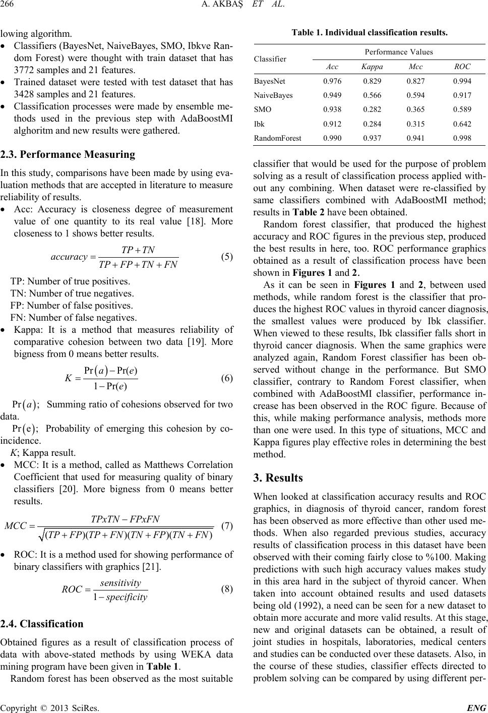

A. AKBAŞ ET AL.

266

lowing algorithm.

• Classifiers (BayesNet, NaiveBayes, SMO , Ibkve Ran -

dom Forest) were thought with train dataset that has

3772 samples and 21 features.

• Trained dataset were tested with test dataset that has

3428 samples and 21 features.

• Classification processes were made by ensemble me-

thods used in the previous step with AdaBoostMI

alghoritm and new results were gathe r ed.

2.3. Performance Measuring

In this study, comparisons have been made by using eva-

luation methods that are accepted in literature to measure

reliability of results.

• Acc: Accuracy is closeness degree of measurement

value of one quantity to its real value [18]. More

closeness to 1 shows better results.

TP TN

accuracy TPFP TNFN

=+++

(5)

TP: Number of true positives.

TN: Num be r o f t r ue ne ga t ives.

FP: Number of false positives.

FN: Number o f fal s e negative s.

• Kappa: It is a method that measures reliability of

comparative cohesion between two data [19]. More

bigness from 0 means better results.

( )

PrPr()

1Pr( )

−

=−

(6)

( )

Pr ;a

Summing ratio of cohesions observed for two

data.

( )

Pre ;

Probability of emerging this cohesion by co-

incidence.

K; Kappa result.

• MCC: It is a method, called as Matthews Correlation

Coefficient that used for measuring quality of binary

classifiers [20]. More bigness from 0 means better

results.

()( )( )()

TPxTN FPxFN

MCC TPFP TPFNTNFP TNFN

−

=++ ++

(7)

• ROC: It is a method used for showing performance of

binary classifiers with graphics [21].

sensitivity

ROC specificity

=−

(8 )

2.4. Classification

Obtained figures as a result of classification process of

data with above-stated methods by using WEKA data

mining program have been given in Table 1.

Random forest has been observed as the most suitable

Table 1. Individual classification results.

Classif ie r

Performance Values

Acc Kappa Mcc ROC

BayesNet

0.976 0.829 0.827 0.994

NaiveBayes

0.949 0.566 0.594 0.917

SMO

0.938 0.282 0.365 0.589

Ibk

0.912 0.284 0.315 0.642

RandomForest

0.990 0.937 0.941 0.998

classifier that would be used for the purpose of problem

solving as a result of classification process applied with-

out any combining. When dataset were re-classified by

same classifiers combined with AdaBoostMI method;

results in Table 2 have been obta i ned.

Random forest classifier, that produced the highest

accuracy and ROC figures in the previous step, produced

the best results in here, too. ROC performance graphics

obtained as a result of classification process have been

shown in Figures 1 and 2.

As it can be seen in Figures 1 and 2, between used

methods, while random forest is the classifier that pro-

duces the highest ROC values in thyroid cancer diagnosis,

the smallest values were produced by Ibk classifier.

When viewed to these results, Ibk clas sifier falls short in

thyroid cancer diagnosis. When the same graphics were

analyzed again, Random Forest classifier has been ob-

served without change in the performance. But SMO

classifier, contrary to Random Forest classifier, when

combined with AdaBoostMI classifier, performance in-

crease has been observed in the ROC figure. Because of

this, while making performance analysis, methods more

than one were used. In this type of situations, MCC and

Kappa figures play effective roles in d etermining the b est

method.

3. Results

When looked at classification accuracy results and ROC

graphics, in diagnosis of thyroid cancer, random forest

has been observed as more effective than other used me-

thods. When also regarded previous studies, accuracy

results of classification process in this dataset have been

observed with their coming fairly close to %100. Making

predictions with such high accuracy values makes study

in this area hard in the subject of thyroid cancer. When

taken into account obtained results and used datasets

being old ( 1992), a need can be seen for a new dataset to

obtain more accurate and more valid results. At this stage,

new and original datasets can be obtained, a result of

joint studies in hospitals, laboratories, medical centers

and studies can be conducted over these datasets. Also, in

the course of these studies, classifier effects directed to

problem solving can be compared by using different per-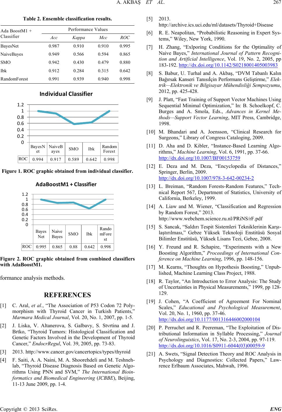

A. AKBAŞ ET AL.

267

Table 2. Ensemble classification results.

Ada BoostM1 +

Classif ie r

Performance Values

Acc Kappa Mcc ROC

BayesNet

0.987 0.910 0.910 0.995

NaiveBayes

0.949 0.566 0.594 0.865

SMO

0.942 0.430 0.479 0.880

Ibk

0.912 0.284 0.315 0.642

RandomForest

0.991 0.939 0.940 0.998

Figure 1. ROC graphic obtained from individual classifier.

Figure 2. ROC graphic obtained from combined classifiers

with AdaBoostM1.

formance analysis methods.

REFERENCES

[1] C. Aral, et al., “The Association of P53 Codon 72 Poly-

morphism with Thyroid Cancer in Turkish Patients,”

Marmara Medical Journal, Vol. 20, No. 1, 2007, pp. 1-5.

[2] J. Liska, V. Altanerova, S. Galbavy, S. Stvrtina and J.

Brtko, “Thyroid Tumors: Histological Classification and

Genetic Factors Involved in the Development of Thyroid

Cancer,” EndocrRegul, Vol. 39, 2005, pp. 73-83.

[3] 2013. http://www.cancer.gov/cancertopics/types/thyroid

[4] F. Saiti, A. A. Naini , M. A. Shoorehdeli and M. Teshneh-

lab, “Thyroid Disease Diagnosis Based on Genetic Algo-

rithms Using PNN and SVM,” The International Bioin-

formatics and Biomedical Engineering (ICBBE), Beijing,

11-13 June 2009, pp. 1-4.

[5] 2013.

http://archive.ics.uci.edu/ml/datasets/Thyroid+Disease

[6] R. E. Neapolitan, “Probabilistic Reasoning in Expert Sys-

tems,” Wiley, New York, 1990.

[7] H. Zhang, “Exlporing Conditions for the Optimality of

Naive Bayes,” International Journal of Pattern Recogni-

tion and Artificial Intelligence, Vol. 19, No. 2, 2005, pp

183-192. http://dx.doi.org/10.1142/S0218001405003983

[8] S. Babur, U. Turhal and A. Akbaş, “DVM Tabanlı Kalın

Bağırsak Kanseri Tanısıİçin Performans Geliştirme,” Elek-

trik—Elektronik ve Bilgisayar Mühendisliği Sempozyumu,

2012, pp. 425-428.

[9] J. Platt, “Fast Training of Support Vector Machines Using

Sequential Minimal Optimization,” In: B. Schoelkopf, C.

Burges and A. Smola, Eds., Advances in Kernel Me-

thods—Support Vector Learning, MIT Press, Cambridge,

1998.

[10] M. Bhandari and A. Joensson, “Clinical Research for

Surgeons,” Library of Congress Cataloging, 2009.

[11] D. Aha and D. Kibler, “Instance-Based Learning Algo-

rithms,” Machine Learning, Vol. 6, 1991, pp. 37-66.

http://dx.doi.org/10.1007/BF00153759

[12] E. Deza and M. Deza, “Encyclopedia of Distances,”

Springer, Berlin, 2009.

http://dx.doi.org/10.1007/978-3-642-00234-2

[13] L. Breiman, “Random Forests-Random Features,” Tech-

nical Report 567, Department of Statistics, University of

California, Berkeley, 1999.

[14] A. Liaw and M. Wiener, “Classification and Regression

by Random Forest,” 2013.

http://www.webchem.science.ru.nl/PRiNS/rF.pdf

[15] S. Sancak, “Saldırı Tespit Sistemleri Tekniklerinin Karşı-

laştırılması,” Gebze Yüksek Teknoloji Enstitüsü S osy a l

Bilimler Enstitüsü, Yüksek Lisans Tezi, Gebze, 2008.

[16] Y. Freund and R. Schapire, “Experiments with a New

Boosting Algorithm,” Proceedings of International Con-

ference on Machine Learning, 1996, pp. 148-156.

[17] M. Kearns, “Thoughts on Hypothesis Boosting,” Unpub-

lished, Machine Learning Class Project, 1988.

[18] R. Taylor, “An Introduction to Error Analysis: The Study

of Uncertainties in Physical Measurements,” 1999, pp 128-

129.

[19] J. Cohen, “A Coefficient of Agreement For Nominal

Scales,” Educational and Psychological Measurement,

Vol. 20, No. 1, 1960, pp. 37-46.

http://dx.doi.org/10.1177/001316446002000104

[20] P. Perruchet and R. Peereman, “The Exploitation of Dis-

tributional Information in Syllable Processing,” Journal

of Neurolinguistics, Vol. 17, No. 2-3, 2004, pp. 97-119.

http://dx.doi.org/10.1016/S0911-6044(03)00059-9

[21] A. Swets, “Signal Detect ion Theory and ROC Analysis in

Psychology and Diagnostics: Collected Papers,” Law-

rence Erlbaum Associates, Mahwah, 1996.

BayesN

NaiveB

ay es

SMO

Ibk

Random

Forest

RO C

0.994

0.917

0.589

0.642

0.998

0.2

0.4

0.6

0.8

1.2

Individual Classifier

Bayes

Net

Naive

Bayes

SMO

Ibk

Rando

mFore

ROC

0.995

0.865

0.88

0.642

0.998

0.2

0.4

0.6

0.8

1.2

AdaBoostM1 + Classifier