Optimal Placement of Distributed Generation for Reliability Benefit in Distribution Systems

doi:10.4236/epe.2013.54B132

Paper Menu >>

Journal Menu >>

Energy and Power Engineering, 2013, 5, 683-688

doi:10.4236/epe.2013.54B132 Published Online July 2013 (http://www.scirp.org/journal/epe)

Optimal Placement of Distributed Generation for

Reliability Benefit in Distribution Systems

N. Rugthaicharoencheep, A. Chalangsut

Department of Electrical Engineering, Faculty of Engineering, Rajamangala University of Technology Phra Nakhon,

Bangkok, Thailand

Email: [email protected]

Received February, 2013

ABSTRACT

A distributed generator is a small-scaled active generating unit located on or near the site where it is to be used. Several

benefits have been realized by installing distributed generators in a distribution network. Among them is reliability im-

provement if their locations and sizes are appropriately determined. For this reason, reliability benefit is investigated in

this paper with the main objective for the optimal placement and sizing of distributed generators in a distribution system

to minimize the customer interruption cost subject to the maximum number of distributed generators, total capacity of

distributed generators, bus voltage limits, current transfer capability of the feeders and only one distributed generator

for one installation position. The technique employed to solve the minimization problem is based on a developed Tabu

search algorithm and reliability worth analysis. The Tabu search algorithm is a local search that uses memory to avoid

being trapped around a local neighborhood and help to move away from a local optimum solution. The reliability worth

analysis provides an indirect measure for cost implication associated with power failure. The developed methodology is

tested with a distribution system of Provincial Electricity Authority (PEA). Numerical results from the tests demonstrate

that distributed generators can be used to promote the reliability of the distribution system.

Keywords: Distributed Generation; Reliability; Tabu Search; Distribution System

1. Introduction

Electricity has always been the major part of human de-

velopment and it has gone through various changes with

time. Traditionally, much of the electricity generated has

been produced by large-scaled, centralized power plants

using fossil fuels (e.g., coal, oil and gas), hydropower or

nuclear power. The electrical energy is transmitted over

long distances by extra high voltage (EHV) or ultra high

voltage (UHV) transmission lines and from there the

high voltage levels are converted to low voltage levels

through distribution lines in the distribution system to

end-use customers [1].

Such a centralized generation pattern, however, suffers

a number of drawbacks, such as a high level of depend-

ence on imported fuels that are very vulnerable, trans-

mission losses, the necessity for continuous upgrading

and replacement of the transmission and distribution fa-

cilities and therefore high operating cost, and environ-

mental impact. In addition, as electric demand is substan-

tially increasing as a result of economic and social

growths, the construction of a large sized power plant is

running into financial and technical difficulties, because

it is capital intensive and needs considerable amount of

time.

An ideal alternative on electric distributions to electric

users is the installation of a small sized generator or

commonly known as distributed generator (DG). DG is a

small-scale active generating unit located on or near the

site where it is to be used (i.e., in distribution systems).

The primary energy resources of DG could be wind, so-

lar, biomass, fuel cells and hydrogen, etc [2].

Although DGs have gained many positive effects, they

still have some economic and technical issues to be ad-

dressed before their applications in the distribution sys-

tem can be realized. The main objective of this paper is

to investigate the impact of distributed generation on

distribution system reliability. It is expected that reliabil-

ity on the installation of DGs can be improved because

they can be served as backup generation when a utility

supply interruption occurs. In other words, some of the

load points can still be electrically supplied by the DGs

and therefore economic loss as a result of the power out-

age can be reduced. However, amount of reliability im-

provement depends on location and size of the DGs to be

installed. It is therefore proposed in this paper a method

to determine the optimal placement and sizing of DGs in

a distribution system to minimize the customer interrup-

tion cost subject to system operational constraints [3].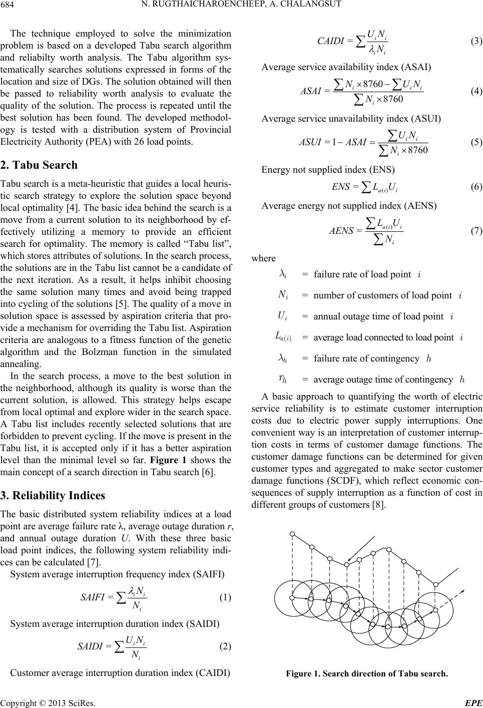

N. RUGTHAICHAROENCHEEP, A. CHALANGSUT

684

The technique employed to solve the minimization

problem is based on a developed Tabu search algorithm

and reliabilty worth analysis. The Tabu algorithm sys-

tematically searches solutions expressed in forms of the

location and size of DGs. The solution obtained will then

be passed to reliability worth analysis to evaluate the

quality of the solution. The process is repeated until the

best solution has been found. The developed methodol-

ogy is tested with a distribution system of Provincial

Electricity Authority (PEA) with 26 load points.

2. Tabu Search

Tabu search is a meta-heuristic that guides a local heuris-

tic search strategy to explore the solution space beyond

local optimality [4]. The basic idea behind the search is a

move from a current solution to its neighborhood by ef-

fectively utilizing a memory to provide an efficient

search for optimality. The memory is called “Tabu list”,

which stores attributes of solutions. In the search process,

the solutions are in the Tabu list cannot be a candidate of

the next iteration. As a result, it helps inhibit choosing

the same solution many times and avoid being trapped

into cycling of the solutions [5]. The quality of a move in

solution space is assessed by aspiration criteria that pro-

vide a mechanism for overriding the Tabu list. Aspiration

criteria are analogous to a fitness function of the genetic

algorithm and the Bolzman function in the simulated

annealing.

In the search process, a move to the best solution in

the neighborhood, although its quality is worse than the

current solution, is allowed. This strategy helps escape

from local optimal and explore wider in the search space.

A Tabu list includes recently selected solutions that are

forbidden to prevent cycling. If the move is present in the

Tabu list, it is accepted only if it has a better aspiration

level than the minimal level so far. Figure 1 shows the

main concept of a search direction in Tabu search [6].

3. Reliability Indices

The basic distributed system reliability indices at a load

point are average failure rate λ, average outage duration r,

and annual outage duration U. With these three basic

load point indices, the following system reliability indi-

ces can be calculated [7].

System average interruption frequency index (SAIFI)

=ii

SAIFI N



 (1)

System average interruption duration index (SAIDI)

=ii

SAIDI N

 (2)

Customer average interruption duration index (CAIDI)

=ii

CAIDI N



 (3)

Average service availability index (ASAI)

8760

=8760

ASAI N







 (4)

Average service unavailability index (ASUI)

=1 8760

ASUIASAI N





 (5)

Energy not supplied index (ENS)

()

=ai i

ENSL U



(6)

Average energy not supplied index (AENS)

()

=ai i

AENS N



 (7)

where

l =failure rate of load point

N =number of customers of load point

U =annual outage time of load point

()ai

L=average load connected to load point

l =failure rate of contingency

r =average outage time of contingency

A basic approach to quantifying the worth of electric

service reliability is to estimate customer interruption

costs due to electric power supply interruptions. One

convenient way is an interpretation of customer interrup-

tion costs in terms of customer damage functions. The

customer damage functions can be determined for given

customer types and aggregated to make sector customer

damage functions (SCDF), which reflect economic con-

sequences of supply interruption as a function of cost in

different groups of customers [8].

Figure 1. Search direction of Tabu search.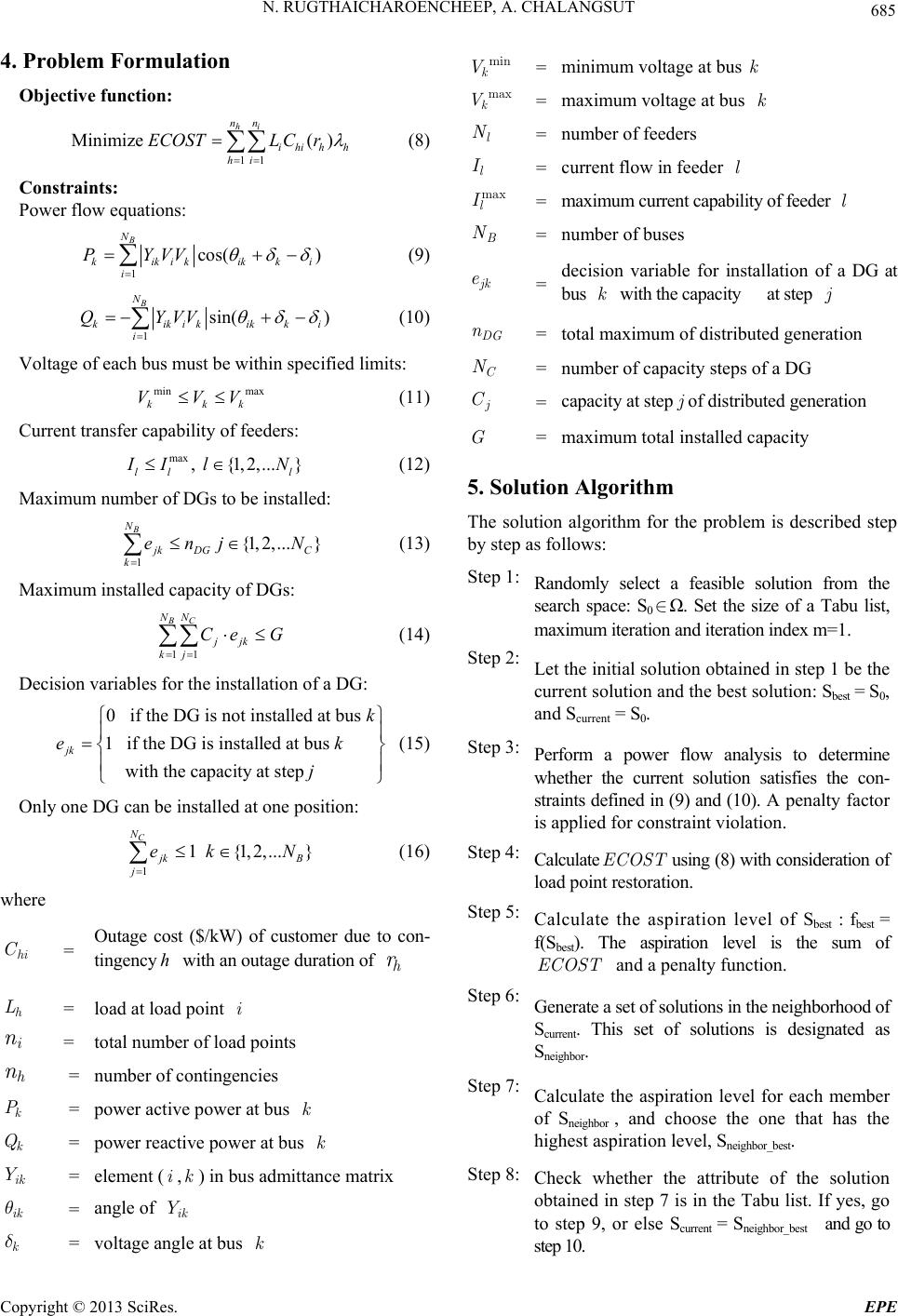

N. RUGTHAICHAROENCHEEP, A. CHALANGSUT 685

4. Problem Formulation

Objective f unction:

Minimize ()

ihih h

ECOSTLC r





 (8)

Constraints:

Power flow equations:

cos( )

kikikikk

PYVV i









 (9)

sin( )

kikikikk

QYVV i







 

 (10)

Voltage of each bus must be within specified limits:

min max

kkk

VVV (11)

Current transfer capability of feeders:

max , {1,2,...}

ll l

Il N (12)

Maximum number of DGs to be installed:

{1,2,...}

kDG C

enj N





 (13)

Maximum installed capacity of DGs:

jjk

Ce G







 (14)

Decision variables for the installation of a DG:

0 if the DG is not installed at bus

1 if the DG is installed at bus

with the capacity at step



















(15)

Only one DG can be installed at one position:

1 {1,2,...}

ek N





B

(16)

where

C = Outage cost ($/kW) of customer due to con-

tingency with an outage duration of

L = load at load point

n = total number of load points

n = number of contingencies

P = power active power at bus

Q = power reactive power at bus

Y = element (i,k) in bus admittance matrix

q = angle of

d = voltage angle at bus

min

V=minimum voltage at bus k

max

V=maximum voltage at bus

N =number of feeders

I =current flow in feeder

max

I=maximum current capability of feeder

N =number of buses

e =decision variable for installation of a DG at

bus with the capacity at step

n =total maximum of distributed generation

N =number of capacity steps of a DG

C =capacity at stepof distributed generation

G =

maximum total installed capacity

5. Solution Algorithm

The solution algorithm for the problem is described step

by step as follows:

Step 1:Randomly select a feasible solution from the

search space: S0ÎΩ. Set the size of a Tabu list,

maximum iteration and iteration index m=1.

Step 2:Let the initial solution obtained in step 1 be the

current solution and the best solution: Sbest = S0,

and Scurrent = S0.

Step 3:Perform a power flow analysis to determine

whether the current solution satisfies the con-

straints defined in (9) and (10). A penalty factor

is applied for constraint violation.

Step 4:Calculate EC using (8) with consideration of

load point restoration.

OST

Step 5:Calculate the aspiration level of Sbest : fbest =

f(Sbest). The aspiration level is the sum of

and a penalty function.

ECOST

Step 6:G enerate a set of solutions in the neighborhood of

Scurrent. This set of solutions is designated as

Sneighbor.

Step 7:Calculate the aspiration level for each member

of Sneighbor , and choose the one that has the

highest aspiration level, Sneighbor_best.

Step 8:Check whether the attribute of the solution

obtained in step 7 is in the Tabu list. If yes, go

to step 9, or else Scurrent = Sneighbor_best and go to

step 10.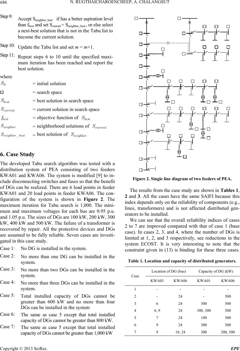

N. RUGTHAICHAROENCHEEP, A. CHALANGSUT

686

Step 9: Accept Sneighbor_best if has a better aspiration level

than fbest and set Scurrent = Sneighbor_best , or else select

a next-best solution that is not in the Tabu list to

become the current solution.

Step 10: Update the Tabu list and set m = m+1.

Step 11: Repeat steps 6 to 10 until the specified maxi-

mum iteration has been reached and report the

best solution.

where

S = initial solution

Ω = search space

best

S = best solution in search space

current

S = current solution in search space

best

= objective function of

best

neighbor

S = neighborhood solutions of

current

_neighborbest

S = best solution of

neighbor

6. Case Study

The developed Tabu search algorithm was tested with a

distribution system of PEA consisting of two feeders

KWA01 and KWA06. The system is modified [9] to in-

clude disconnecting switches and fuses so that the benefit

of DGs can be realized. There are 6 load points in feeder

KWA01 and 20 load points in feeder KWA06. The con-

figuration of the system is shown in Figure 2. The

maximum iteration for Tabu search is 1,000. The mini-

mum and maximum voltages for each bus are 0.95 p.u.

and 1.05 p.u. The sizes of DGs are 100 kW, 200 kW, 300

kW, 400 kW and 500 kW. The failure of a transformer is

recovered by repair. All the protective devices and DGs

are assumed to be fully reliable. Seven cases are investi-

gated in this case study.

Case 1: No DG is installed in the system.

Case 2:

o more than one DG can be installed in the

system.

Case 3: No more than two DGs can be installed in the

system.

Case 4:

o more than three DGs can be installed in the

system.

Case 5: Total installed capacity of DGs cannot be

greater than 600 kW and no more than fou

DGs can be installed in the system

Case 6: The same as case 5 except that total installe

capacity of DGs cannot be greater than 800 kW.

Case 7: The same as case 5 except that total installed

capacity of DGs cannot be greater than 1,000 kW

Figure 2. Single line diagram of two feeders of PEA.

The results from the case study are shown in Tab le s 1,

2 and 3. All the cases have the same SAIFI because this

index depends only on the reliability of components (e.g.,

lines, transformers) and is not affected distributed gen-

erators to be installed.

We can see that the overall reliability indices of cases

2 to 7 are improved compared with that of case 1 (base

case). In cases 2, 3, and 4, where the number of DGs is

limited at 1, 2, and 3 respectively, see reductions in the

system ECOST. It is very interesting to note that the

constraint given in (13) is binding for these three cases.

Table 1. Location and capacity of distributed generators.

Location of DG (bus) Capacity of DG (kW)

Case

KWA01 KWA06 KWA01 KWA06

1 - - - -

2 - 24 - 500

3 6 24 300 500

4 6, 9 24 300, 300 500

5 7 24 100 500

6 9 24 300 500

7 9 18, 24 300 200, 500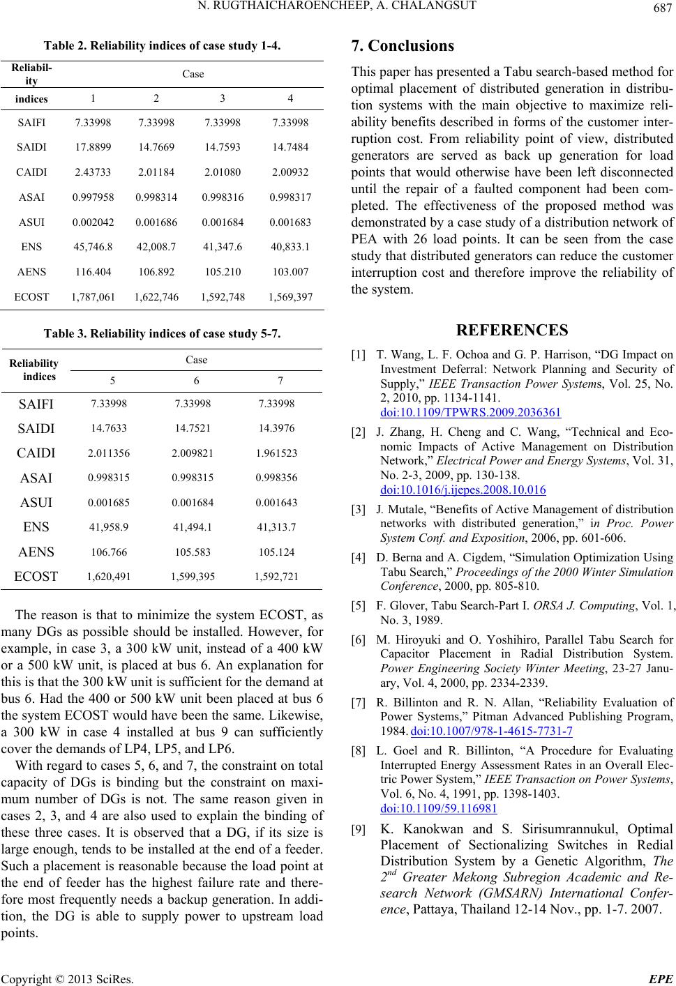

N. RUGTHAICHAROENCHEEP, A. CHALANGSUT 687

Table 2. Reliability indices of case study 1-4.

Reliabil-

ity Case

indices 1 2 3 4

SAIFI 7.33998 7.33998 7.33998 7.33998

SAIDI 17.8899 14.7669 14.7593 14.7484

CAIDI 2.43733 2.01184 2.01080 2.00932

ASAI 0.997958 0.998314 0.998316 0.998317

ASUI 0.002042 0.001686 0.001684 0.001683

ENS 45,746.8 42,008.7 41,347.6 40,833.1

AENS 116.404 106.892 105.210 103.007

ECOST 1,787,061 1,622,746 1,592,748 1,569,397

Table 3. Reliability indices of case study 5-7.

Case

Reliability

indices 5 6 7

SAIFI 7.33998 7.33998 7.33998

SAIDI 14.7633 14.7521 14.3976

CAIDI 2.011356 2.009821 1.961523

ASAI 0.998315 0.998315 0.998356

ASUI 0.001685 0.001684 0.001643

ENS 41,958.9 41,494.1 41,313.7

AENS 106.766 105.583 105.124

ECOST 1,620,491 1,599,395 1,592,721

The reason is that to minimize the system ECOST, as

many DGs as possible should be installed. However, for

example, in case 3, a 300 kW unit, instead of a 400 kW

or a 500 kW unit, is placed at bus 6. An explanation for

this is that the 300 kW unit is sufficient for the demand at

bus 6. Had the 400 or 500 kW unit been placed at bus 6

the system ECOST would have been the same. Likewise,

a 300 kW in case 4 installed at bus 9 can sufficiently

cover the demands of LP4, LP5, and LP6.

With regard to cases 5, 6, and 7, the constraint on total

capacity of DGs is binding but the constraint on maxi-

mum number of DGs is not. The same reason given in

cases 2, 3, and 4 are also used to explain the binding of

these three cases. It is observed that a DG, if its size is

large enough, tends to be installed at the end of a feeder.

Such a placement is reasonable because the load point at

the end of feeder has the highest failure rate and there-

fore most frequently needs a backup generation. In addi-

tion, the DG is able to supply power to upstream load

points.

7. Conclusions

This paper has presented a Tabu search-based method for

optimal placement of distributed generation in distribu-

tion systems with the main objective to maximize reli-

ability benefits described in forms of the customer inter-

ruption cost. From reliability point of view, distributed

generators are served as back up generation for load

points that would otherwise have been left disconnected

until the repair of a faulted component had been com-

pleted. The effectiveness of the proposed method was

demonstrated by a case study of a distribution network of

PEA with 26 load points. It can be seen from the case

study that distributed generators can reduce the customer

interruption cost and therefore improve the reliability of

the system.

REFERENCES

[1] T. Wang, L. F. Ochoa and G. P. Harrison, “DG Impact on

Investment Deferral: Network Planning and Security of

Supply,” IEEE Transaction Power Systems, Vol. 25, No.

2, 2010, pp. 1134-1141.

doi:10.1109/TPWRS.2009.2036361

[2] J. Zhang, H. Cheng and C. Wang, “Technical and Eco-

nomic Impacts of Active Management on Distribution

Network,” Electrical Power and Energy Systems, Vol. 31,

No. 2-3, 2009, pp. 130-138.

doi:10.1016/j.ijepes.2008.10.016

[3] J. Mutale, “Benefits of Active Management of distribution

networks with distributed generation,” in Proc. Power

System Conf. and Exposition, 2006, pp. 601-606.

[4] D. Berna and A. Cigdem, “Simulation Optimization Using

Tabu Search,” Proceedings of the 2000 Winter Simulation

Conference, 2000, pp. 805-810.

[5] F. Glover, Tabu Search-Part I. ORSA J. Computing, Vol. 1,

No. 3, 1989.

[6] M. Hiroyuki and O. Yoshihiro, Parallel Tabu Search for

Capacitor Placement in Radial Distribution System.

Power Engineering Society Winter Meeting, 23-27 Janu-

ary, Vol. 4, 2000, pp. 2334-2339.

[7] R. Billinton and R. N. Allan, “Reliability Evaluation of

Power Systems,” Pitman Advanced Publishing Program,

1984. doi:10.1007/978-1-4615-7731-7

[8] L. Goel and R. Billinton, “A Procedure for Evaluating

Interrupted Energy Assessment Rates in an Overall Elec-

tric Power System,” IEEE Transaction on Power Systems,

Vol. 6, No. 4, 1991, pp. 1398-1403.

doi:10.1109/59.116981

[9] K. Kanokwan and S. Sirisumrannukul, Optimal

Placement of Sectionalizing Switches in Redial

Distribution System by a Genetic Algorithm, The

2nd Greater Mekong Subregion Academic and Re-

search Network (GMSARN) International Confer-

ence, Pattaya, Thailand 12-14 Nov., pp. 1-7. 2007.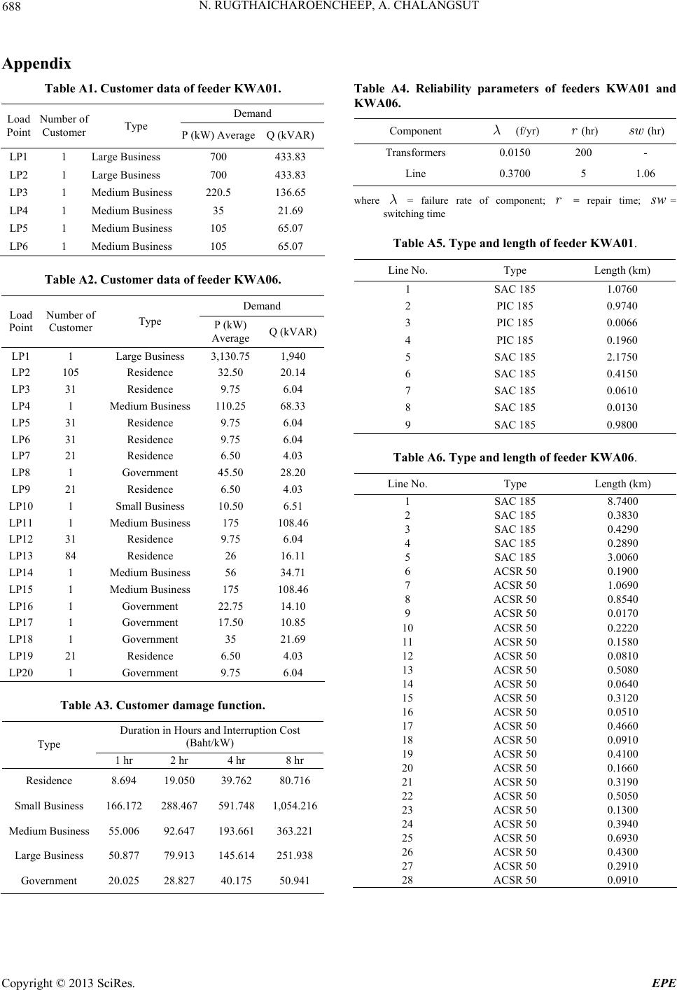

N. RUGTHAICHAROENCHEEP, A. CHALANGSUT

688

Appendix

Table A1. Customer data of feeder KWA01. Table A4. Reliability parameters of feeders KWA01 and

KWA06.

Demand

Load

Point

Number of

Customer Type P (kW) Average Q (kVAR)

LP1 1 Large Business 700 433.83

LP2 1 Large Business 700 433.83

LP3 1 Medium Business220.5 136.65

LP4 1 Medium Business35 21.69

LP5 1 Medium Business105 65.07

LP6 1 Medium Business105 65.07

Component l (f/yr) r(hr) sw (hr)

Transformers 0.0150 200 -

Line 0.3700 5 1.06

where = failure rate of component; r = repair time; l

switching time

Table A5. Type and length of feeder KWA01.

Line No. Type Length (km)

1 SAC 185 1.0760

2 PIC 185 0.9740

3 PIC 185 0.0066

4 PIC 185 0.1960

5 SAC 185 2.1750

6 SAC 185 0.4150

7 SAC 185 0.0610

8 SAC 185 0.0130

9 SAC 185 0.9800

Table A2. Customer data of feeder KWA06.

Demand

Load

Point

Number of

Customer Type P (kW)

Average Q (kVAR)

LP1 1 Large Business 3,130.75 1,940

LP2 105 Residence 32.50 20.14

LP3 31 Residence 9.75 6.04

LP4 1 Medium Business 110.25 68.33

LP5 31 Residence 9.75 6.04

LP6 31 Residence 9.75 6.04

LP7 21 Residence 6.50 4.03

LP8 1 Government 45.50 28.20

LP9 21 Residence 6.50 4.03

LP10 1 Small Business 10.50 6.51

LP11 1 Medium Business 175 108.46

LP12 31 Residence 9.75 6.04

LP13 84 Residence 26 16.11

LP14 1 Medium Business 56 34.71

LP15 1 Medium Business 175 108.46

LP16 1 Government 22.75 14.10

LP17 1 Government 17.50 10.85

LP18 1 Government 35 21.69

LP19 21 Residence 6.50 4.03

LP20 1 Government 9.75 6.04

Table A6. Type and length of feeder KWA06.

Line No. Type Length (km)

1 SAC 185 8.7400

2 SAC 185 0.3830

3 SAC 185 0.4290

4 SAC 185 0.2890

5 SAC 185 3.0060

6 ACSR 50 0.1900

7 ACSR 50 1.0690

8 ACSR 50 0.8540

9 ACSR 50 0.0170

10 ACSR 50 0.2220

11 ACSR 50 0.1580

12 ACSR 50 0.0810

13 ACSR 50 0.5080

14 ACSR 50 0.0640

15 ACSR 50 0.3120

16 ACSR 50 0.0510

17 ACSR 50 0.4660

18 ACSR 50 0.0910

19 ACSR 50 0.4100

20 ACSR 50 0.1660

21 ACSR 50 0.3190

22 ACSR 50 0.5050

23 ACSR 50 0.1300

24 ACSR 50 0.3940

25 ACSR 50 0.6930

26 ACSR 50 0.4300

27 ACSR 50 0.2910

28 ACSR 50 0.0910

Table A3. Customer damage function.

Duration in Hours and Interruption Cost

(Baht/kW)

Type

1 hr 2 hr 4 hr 8 hr

Residence 8.694 19.050 39.762 80.716

Small Business 166.172 288.467 591.748 1,054.216

Medium Business 55.006 92.647 193.661 363.221

Large Business 50.877 79.913 145.614 251.938

Government 20.025 28.827 40.175 50.941