

Paper Menu >>
Journal Menu >>
 Vol.3, No.4, 314-320 (2013) Open Journal of Animal Sciences http://dx.doi.org/10.4236/ojas.2013.34047 Relating models of activity metabolism to the metabolic efficiency of steady swimming Anthony Papadopoulos Natural Sciences Department, St. Petersburg College, Tarpon Springs, USA; [email protected] Received 2 September 2013; revised 5 October 2013; accepted 17 October 2013 Copyright © 2013 Anthony Papadopoulos. This is an open access article distributed under the Creative Commons Attribution License, which permits unrestricted use, distribution, and reproduction in any medium, provided the original work is properly cited. ABSTRACT Power-law () and exponential power-law () functional forms model activity metabo- lism (U) for fully submerged swimming ani- mals, and are special cases of the power-law polynomial equation, c abU+ qUc ae M c ψ c UqUc abU ψ Ma abUψ ae -1 if =1 =1+ =if + in which U is the observed total metabolic rate measured at an observed steady swimming speed, . The relationship between the meta- bolic efficiency of steady swimming and the exponents of U is addressed in this paper to establish the use of (for c) and (for ) as optimal efficiencies for comparing the hydrodynamic and muscle metabolic efficien- cies among fully submerged animals that en- gage in steady swimming activities. The meta- bolic efficiency of steady swimming is trans- formed into its ideal form ( M U M c-1 >1 ˆ U ψ-1 ψ>1 η ) from which the optimal hydrodynamic efficiency () and the optimal muscle metabolic efficiency ( ˆh= η c-1 ˆ= m η -1 ψ ) are derived. These optimal efficien- cies are therefore ideal metabolic efficiencies measured at different optimal steady speeds. Subsequently, linear () and exponential () models are approximations with diver- gent optimal muscle metabolic efficiencies ( and , respectively), but with a similar optimal hydrodynamic efficiency ( + abU qU ae ˆm η 1ˆm η 1ˆ η h 1). Keywords: Activity Metabolism; Exponent; Metabolic Efficiency; Power Law; Steady Swimming 1. INTRODUCTION The activity metabolism (U M ) of a swimming animal is the observed rate of total metabolic energy measured at an observed steady swimming speed, . The func- tional forms that model U U M for a fully submerged animal are exponential () and power law () [1-7]. Both forms, however, are special cases of the power-law polynomial equation [8], qU ae c abU 1if 1 1 if c c UqU c abU MaabU ae (1) in which the coefficients (a, b, c, and ) are hydrody- namical and physiological descriptors (see [7,8] for de- tails). Note: 11 and .bqa An important question that has not been addressed in the literature is how the swim-speed exponent (c) and the metabolic exponent ( ) analytically relate to efficien- cies. Experimental evidence suggests that c in 1 U M is a useful coefficient for comparing the swimming effi- ciency among different animals [9-14]. Papadopoulos [8] proposes that c in Equation (1) relates inversely to the propulsive (or hydrodynamic) efficiency of steady swim- ming and that ψ relates inversely to the metabolic con- version (or muscle metabolic) efficiency of steady swim- ming. But there is no analytical formulation that explic- itly shows how c or ψ relates to efficiency. Although there is experimental evidence that suggests an inverse association between c and swimming efficiency, the de- finitive correspondence should be derived analytically from theory. And this also applies to the metabolic ex- ponent, ψ. This paper addresses the analytical relationship be- tween the metabolic efficiency of steady swimming and the exponents of Equation (1). The analysis confirms that 1 c (for c) is the optimal hydrodynamic efficiency of an animal in its ideal steady swimming state and that 1 1 (for 1 ) is the optimal muscle metabolic effi- ciency of an animal in its ideal steady swimming state. Copyright © 2013 SciRes. OPEN ACCESS 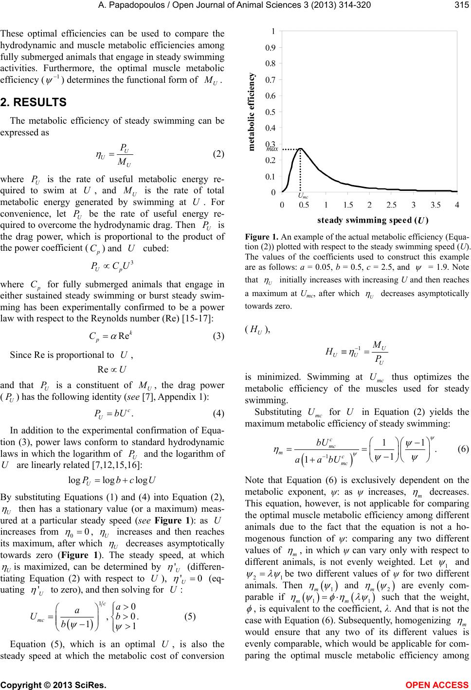 A. Papadopoulos / Open Journal of Animal Sciences 3 (2013) 314-320 315 These optimal efficiencies can be used to compare the hydrodynamic and muscle metabolic efficiencies among fully submerged animals that engage in steady swimming activities. Furthermore, the optimal muscle metabolic efficiency (1 ) determines the functional form of U M . 2. RESULTS The metabolic efficiency of steady swimming can be expressed as U U U P M (2) where U is the rate of useful metabolic energy re- quired to swim at U, and U P M is the rate of total metabolic energy generated by swimming at U. For convenience, let U be the rate of useful energy re- quired to overcome the hydrodynamic drag. Then U is the drag power, which is proportional to the product of the power coefficient ( P P p C) and cubed: U 3 Up PCU where p C for fully submerged animals that engage in either sustained steady swimming or burst steady swim- ming has been experimentally confirmed to be a power law with respect to the Reynolds number (Re) [15-17]: Rek p C (3) Since Re is proportional to , U Re U and that U is a constituent of U P M , the drag power () has the following identity (see [7], Appendix 1): U P . c U PbU (4) In addition to the experimental confirmation of Equa- tion (3), power laws conform to standard hydrodynamic laws in which the logarithm of U and the logarithm of are linearly related [7,12,15,16]: P U loglog log U PbcU By substituting Equations (1) and (4) into Equation (2), U then has a stationary value (or a maximum) meas- ured at a particular steady speed (see Figure 1): as increases from 0 U 0 , U increases and then reaches its maximum, after which U decreases asymptotically towards zero (Figure 1). The steady speed, at which U is maximized, can be determined by 'U (differen- tiating Equation (2) with respect to ), U'0 U (eq- uating 'U to zero), and then solving for : U 10 , 11 c mc a a U b 0 .b (5) Equation (5), which is an optimal U, is also the steady speed at which the metabolic cost of conversion Figure 1. An example of the actual metabolic efficiency (Equa- tion (2)) plotted with respect to the steady swimming speed (U). The values of the coefficients used to construct this example are as follows: a = 0.05, b = 0.5, c = 2.5, and = 1.9. Note that U initially increases with increasing U and then reaches a maximum at Umc, after which U decreases asymptotically towards zero. (U H ), 1U UU U M HP is minimized. Swimming at mc U thus optimizes the metabolic efficiency of the muscles used for steady swimming. Substituting mc for U in Equation (2) yields the maximum metabolic efficiency of steady swimming: U 1 11 . 1 1 c mc mc mc bU aabU (6) Note that Equation (6) is exclusively dependent on the metabolic exponent, ψ: as ψ increases, m decreases. This equation, however, is not applicable for comparing the optimal muscle metabolic efficiency among different animals due to the fact that the equation is not a ho- mogenous function of ψ: comparing any two different values of m , in which ψ can vary only with respect to different animals, is not evenly weighted. Let 1 and 21 be two different values of ψ for two different animals. Then 1m and 2m are evenly com- parable if 11mm such that the weight, , is equivalent to the coefficient, λ. And that is not the case with Equation (6). Subsequently, homogenizing m would ensure that any two of its different values is evenly comparable, which would be applicable for com- paring the optimal muscle metabolic efficiency among Copyright © 2013 SciRes. OPEN ACCESS 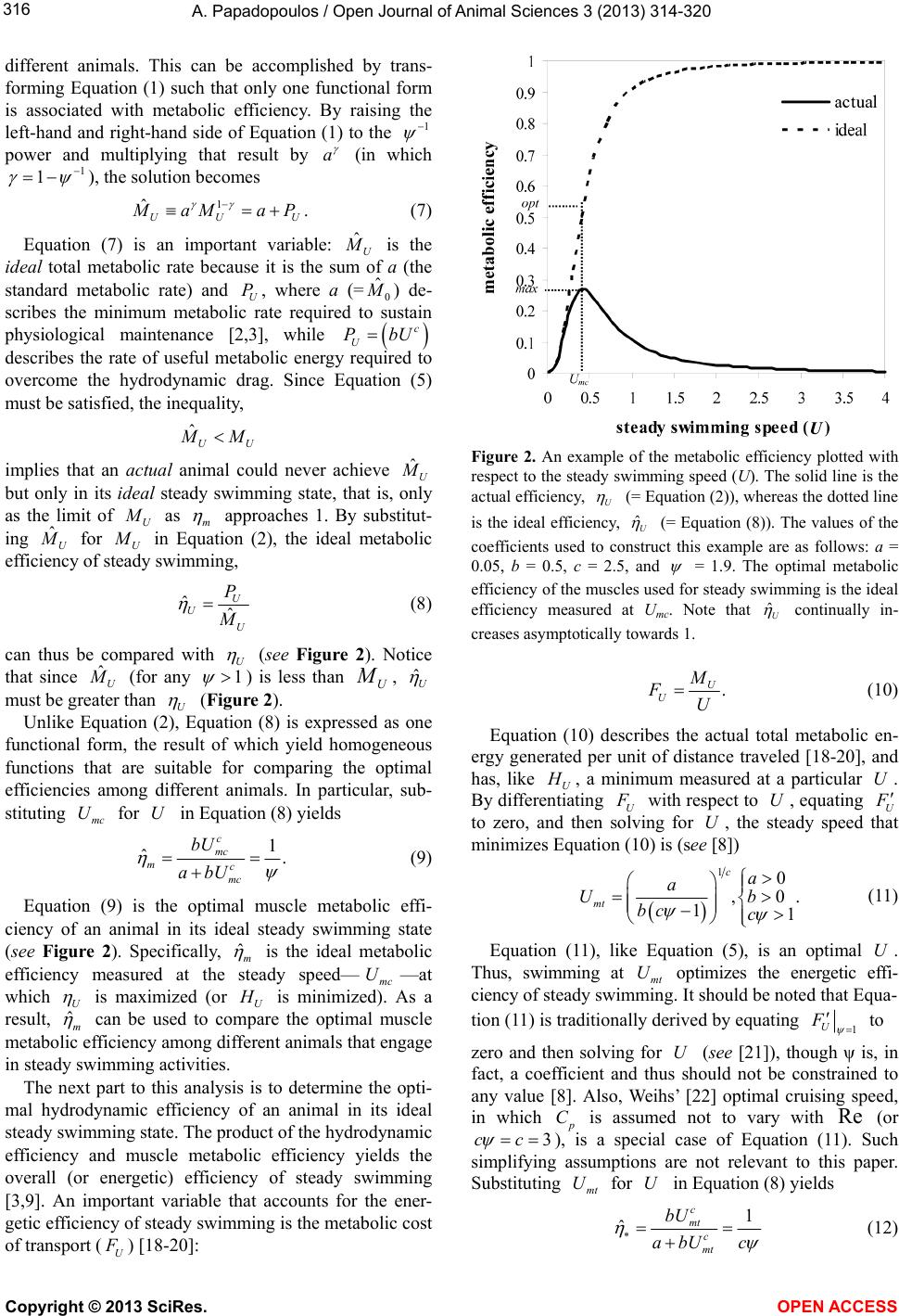 A. Papadopoulos / Open Journal of Animal Sciences 3 (2013) 314-320 316 different animals. This can be accomplished by trans- forming Equation (1) such that only one functional form is associated with metabolic efficiency. By raising the left-hand and right-hand side of Equation (1) to the 1 power and multiplying that result by a (in which 1 1 ), the solution becomes 1 ˆUU U M aMa P . (7) Equation (7) is an important variable: ˆU M is the ideal total metabolic rate because it is the sum of a (the standard metabolic rate) and U, where a (=0 Pˆ M ) de- scribes the minimum metabolic rate required to sustain physiological maintenance [2,3], while c U P bU describes the rate of useful metabolic energy required to overcome the hydrodynamic drag. Since Equation (5) must be satisfied, the inequality, ˆUU M M implies that an actual animal could never achieve ˆU M but only in its ideal steady swimming state, that is, only as the limit of U M as m approaches 1. By substitut- ing ˆU M for U M in Equation (2), the ideal metabolic efficiency of steady swimming, ˆˆ U U U P M (8) can thus be compared with U (see Figure 2). Notice that since ˆU M (for any 1 ) is less than U M , ˆU must be greater than U (Figure 2). Unlike Equation (2), Equation (8) is expressed as one functional form, the result of which yield homogeneous functions that are suitable for comparing the optimal efficiencies among different animals. In particular, sub- stituting for U in Equation (8) yields mc U 1 ˆ. c mc mc mc bU abU (9) Equation (9) is the optimal muscle metabolic effi- ciency of an animal in its ideal steady swimming state (see Figure 2). Specifically, ˆm is the ideal metabolic efficiency measured at the steady speed—mc —at which U U is maximized (or U H is minimized). As a result, ˆm can be used to compare the optimal muscle metabolic efficiency among different animals that engage in steady swimming activities. The next part to this analysis is to determine the opti- mal hydrodynamic efficiency of an animal in its ideal steady swimming state. The product of the hydrodynamic efficiency and muscle metabolic efficiency yields the overall (or energetic) efficiency of steady swimming [3,9]. An important variable that accounts for the ener- getic efficiency of steady swimming is the metabolic cost of transport (U F ) [18-20]: Figure 2. An example of the metabolic efficiency plotted with respect to the steady swimming speed (U). The solid line is the actual efficiency, U (= Equation (2)), whereas the dotted line is the ideal efficiency, ˆU (= Equation (8)). The values of the coefficients used to construct this example are as follows: a = 0.05, b = 0.5, c = 2.5, and = 1.9. The optimal metabolic efficiency of the muscles used for steady swimming is the ideal efficiency measured at Umc. Note that ˆU continually in- creases asymptotically towards 1. . U U M FU (10) Equation (10) describes the actual total metabolic en- ergy generated per unit of distance traveled [18-20], and has, like U H , a minimum measured at a particular . By differentiating U U F with respect to U, equating U F to zero, and then solving for U, the steady speed that minimizes Equation (10) is (see [8]) 10 ,0 11 c mt a a U bc c .b (11) Equation (11), like Equation (5), is an optimal U. Thus, swimming at mt U optimizes the energetic effi- ciency of steady swimming. It should be noted that Equa- tion (11) is traditionally derived by equating 1 U F to zero and then solving for (see [21]), though ψ is, in fact, a coefficient and thus should not be constrained to any value [8]. Also, Weihs’ [22] optimal cruising speed, in which U p C is assumed not to vary with (or Re 3cc ), is a special case of Equation (11). Such simplifying assumptions are not relevant to this paper. Substituting for U in Equation (8) yields mt U 1 ˆ c mt c mt bU c abU (12) Copyright © 2013 SciRes. OPEN ACCESS  A. Papadopoulos / Open Journal of Animal Sciences 3 (2013) 314-320 317 Equation (12) is the optimal energetic efficiency of an animal in its ideal steady swimming state. Specifically, ˆ is the ideal metabolic efficiency measured at the steady speed—mt —at which U U F is minimized. Therefore, ˆ can be used to compare the optimal en- ergetic efficiency among different animals that engage in steady swimming activities. Since the product of the hy- drodynamic efficiency and muscle metabolic efficiency yields the energetic efficiency of steady swimming (see [3,9]), the optimal hydrodynamic efficiency (ˆh ) of an animal in its ideal steady swimming state can thus be determined by the ratio of ˆ to ˆm : ˆ1 ˆˆ h mc where c is the swim-speed exponent. Alternatively, ˆh can be derived by differentiating the ideal cost of trans- port (ˆU F ), ˆ ˆU U M FU with respect to U, equating ˆ F to zero, solving for , U 10 ˆ, 11 c mt a a U bc c 0 , b (13) and then substituting for U in Equation (8): ˆmt U ˆ1 ˆ. ˆ c mt hc mt bU c abU (14) As a result, Equation (14) is the ideal metabolic effi- ciency measured at the steady speed——at which ˆmt U ˆU F is minimized, and can thus be used to compare the optimal hydrodynamic efficiency among different ani- mals that engage in steady swimming activities. 3. DISCUSSION Steady swimming is observed in animals engaging in ecologically important activities such as competing for limited resources, seeking favorable abiotic conditions, and migration [23-27]. During such activities, an animal swims at an optimal steady speed to minimize its meta- bolic cost. For example, during migration, an animal maximizes its distance per unit of total metabolic energy by swimming at the steady speed (mt U) at which the metabolic cost of transport (U F ) is minimized [22,28]. Thus maximizing the distance per unit of total metabolic energy is essential for optimizing the steady swimming performance during migration. Equally essential, how- ever, is optimizing the steady swimming performance during activities in which maximizing distance is not essential. For example, while competing for limited re- sources within a microhabitat, an animal maximizes its useful metabolic energy per unit of total metabolic en- ergy by swimming at the steady speed (mc U) at which the metabolic cost of conversion (U H ) is minimized. Hence, an animal can optimize its steady swimming per- formance for different activities by swimming at (the steady speed at which mt U U F is minimized) or mc U (the steady speed at which U H is minimized). But there is a fundamental difference between these two objectives: U H , unlike U F , is dimensionless; the inverse of U H is, in fact, the metabolic efficiency of steady swimming, U (= Equation (2); see Figure 1). A transformation of U is then formulated in order to yield optimal efficien- cies that are homogenous functions of c and of dif- ferent animals. This is particularly important when com- paring the optimal efficiencies among different animals. This transformation (see Equation (7)) yields the ideal metabolic efficiency of steady swimming, ˆU (= Equa- tion (8); see Figure 2), for which can be any value greater than 1. The ideal steady swimming state of an animal can thus be interpreted as a special case of Equa- tion (2) in which the maximum metabolic efficiency, m (= Equation (6)), approaches 1. Substituting mt (which is the steady speed that op- timizes the energetic efficiency of steady swimming) for in U UˆU yields the optimal energetic efficiency of an animal in its ideal steady swimming state and is identical with Equation (12): 1 ˆ,1c c , where c and are the exponents in Equation (1), which describes the activity metabolism (U M ) of a fully sub- merged animal engaged in steady swimming. The steady speed that optimizes the metabolic efficiency of the mus- cles used for steady swimming—mc U—is then substi- tuted for in UˆU to yield the optimal muscle meta- bolic efficiency of an animal in its ideal steady swim- ming state (see Figure 2), 1 ˆ,1 m , which is identical with Equation (9). Since the energetic efficiency is the product of the hydrodynamic and muscle metabolic efficiencies [3,9], the optimal hydrodynamic efficiency (ˆh ) is simply the ratio of ˆ to ˆm : ˆ1 ˆ,1 ˆ h m c c , which can also be derived by substituting into ˆU the steady speed () that optimizes the hydrodynamic efficiency of an animal in its ideal steady swimming state (see Equations (13) and (14)). The optimal efficiencies, ˆmt U ˆh and ˆm , can thus be used to compare the hydrody- Copyright © 2013 SciRes. OPEN ACCESS 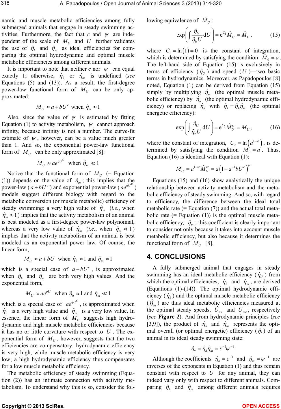 A. Papadopoulos / Open Journal of Animal Sciences 3 (2013) 314-320 318 namic and muscle metabolic efficiencies among fully submerged animals that engage in steady swimming ac- tivities. Furthermore, the fact that c and are inde- pendent of the scale of U M and U further validates the use of ˆh and ˆm as ideal efficiencies for com- paring the optimal hydrodynamic and optimal muscle metabolic efficiencies among different animals. It is important to note that neither c nor can equal exactly 1; otherwise, ˆh or ˆm is undefined (see Equations (5) and (13)). As a result, the first-degree power-law functional form of U M can be only ap- proximated: ˆ 1 Um when c bUMa Also, since the value of is estimated by fitting Equation (1) to activity metabolism, cannot approach infinity, because infinity is not a number. The curve-fit estimate of , however, can be a value much greater than 1. And so, the exponential power-law functional form of U M can be only approximated [8]: ˆ Um wh qU c een 1 Ma Notice that the functional form of U M (= Equation (1)) depends on the value of ˆm ; this implies that the power-law () and exponential power-law () models suggest different biology with regard to the metabolic conversion (or muscle metabolic) efficiency of steady swimming: a very high value of c abUqU c ae ˆm (i.e., when ˆ1 m ) implies that the activity metabolism of an animal is best modeled as a first-degree power-law polynomial, whereas a very low value of ˆm (i.e., when ˆ1 m ) implies that the activity metabolism of an animal is best modeled as an exponential power law. Of course, the linear form, ˆˆ d Uh bU when 1 an1 m Ma which is a special case of , is approximated when c Uab ˆh and ˆm are both very high values. And the exponential form, ˆˆ 1 qU Ma c U e when ae and h 1 m which is a special case of , is approximated when qU ˆh is a very high value and ˆm is a very low value. In essence, the linear form of U M suggests high hydro- dynamic and high muscle metabolic efficiencies because it has no or little curvature with respect to . The ex- ponential form of U U M , however, suggests that the two efficiencies are compensatory: hydrodynamic efficiency is very high, while muscle metabolic efficiency is very low; a high hydrodynamic efficiency thus compensates for a low muscle metabolic efficiency. The metabolic efficiency of steady swimming (Equa- tion (2)) has an intimate connection with activity me- tabolism. To understand why this is so, consider the fol- lowing equivalence of ˆU M : 1 ˆˆˆ expd e, ˆ C U UU h UMM U (15) where 1ln 10C is the constant of integration, which is determined by satisfying the condition 0 ˆ M a . The left-hand side of Equation (15) is exclusively in terms of efficiency (ˆU ) and speed ()—two basic terms in hydrodynamics. Moreover, as Papadopoulos [8] noted, Equation (1) can be derived from Equation (15) simply by multiplying m U ˆ (the optimal muscle meta- bolic efficiency) by ˆh (the optimal hydrodynamic effi- ciency) or replacing ˆh with ˆˆ ˆ hm (the optimal energetic efficiency): 2 ˆˆ expd e, ˆ C U UU UMM U (16) where the constant of integration, , is de- termined by satisfying the condition 0 1 2lnCa M a. Thus, Equation (16) is identical with Equation (1): 11 ˆ1c UU MaMaabU Equations (15) and (16) show analytically the unique relationship between activity metabolism and the meta- bolic efficiency of steady swimming. And so, with regard to efficiency, the difference between the ideal total metabolic rate (= Equation (7)) and the actual total meta- bolic rate (= Equation (1)) is the optimal muscle meta- bolic efficiency, ˆm ; this coefficient is clearly important to consider not only because it takes into account muscle metabolic efficiency, but also because it determines the functional form of U M [8]. 4. CONCLUSIONS A fully submerged animal that engages in steady swimming has an ideal metabolic efficiency ( ˆU ) from which the optimal efficiencies, ˆh and ˆm , are derived (Equations (1)-(14)). The optimal hydrodynamic effi- ciency (ˆh ) and the optimal muscle metabolic efficiency (ˆm ) are thus ideal metabolic efficiencies measured at the optimal steady speeds, U and mc U, respectively (see Figure 2). And from hydrodynamic principles (see [3,9]), the product of ˆmt ˆh and ˆm represents the opti- mal overall (or optimal energetic) efficiency (* ˆ ) of an animal in its ideal steady swimming state: 11 ˆˆˆ . hm c Although the coefficients and 1 ˆhc 1 ˆm are inverses of the exponents in Equation (1) and thus remain constant with respect to U for any animal, they can indeed vary only with respect to different animals. Com- paring ˆh and ˆm among different animals requires Copyright © 2013 SciRes. OPEN ACCESS  A. Papadopoulos / Open Journal of Animal Sciences 3 (2013) 314-320 319 that these optimal efficiencies are homogenous functions of c and : ˆh and ˆm are, in fact, homogenous due to the transformation of Equation (2) into Equation (8), which is the ideal form of U . Furthermore, since ˆh and ˆm are inverses of the exponents in Equation (1), the different models of U M exclusively arise from the different values of ˆh and ˆm . 5. ACKNOWLEDGEMENTS I thank the reviewers for providing comments that improved this manuscript. I was employed at Texas Tech University, where I inde- pendently wrote this manuscript and derived all of the results. Support for this work was provided in part by National Science Foundation award DEB-0616942 to Sean H. Rice. REFERENCES [1] Ivlev, V.S. (1960) Active metabolic intensity in salmon fry (Salmo salar L.) at various rates of activity. Salmon and Trout Comm, Int Counc Explor Sea, Copenhagen, 213, 1-16. [2] Brett, J.R. (1964) The respiratory metabolism and swim- ming performance of young sockeye salmon. Journal of the Fisheries Research Board of Canada, 21, 1183-1226. http://dx.doi.org/10.1139/f64-103 [3] Webb, P.W. (1974) Hydrodynamics and energetics of fish propulsion. Bulletin of the Fisheries Research Board of Canada, 190, 109-119. [4] O’Dor, R.K. and Webber, D.M. (1991) Invertebrate ath- letes: Trade-offs between transport efficiency and power density in cephalopod evolution. The Journal of Experi- mental Biology, 160, 93-112. [5] Hind, A.T. and Gurney, W.S.C. (1997) The metabolic cost of swimming in marine homeotherms. The Journal of Experimental Biology, 200, 531-542. [6] Fish, F.E. (2000) Biomechanics and energetics in aquatic and semiaquatic mammals: Platypus to whale. Physiolo- gical and Biochemical Zoology, 73, 683-698. http://dx.doi.org/10.1086/318108 [7] Papadopoulos, A. (2008) On the hydrodynamics-based power-law function and its application in fish swimming energetics. Transactions of the American Fisheries Soci- ety, 137, 997-1006. http://dx.doi.org/10.1577/T07-116.1 [8] Papadopoulos, A. (2009) Hydrodynamics-based functional forms of activity metabolism: A case for the power-law polynomial function in animal swimming energetics. PLoS ONE, 4, e4852. http://dx.doi.org/10.1371/journal.pone.0004852 [9] Webb, P.W. (1993) Swimming. In: Evens, D.H., Ed., The Physiology of Fishes, CRC Press, Boca Raton, 47-73. [10] Wardle, C.S., Soofiani, N.M., O’Neill, F.G., Glass, C.W. and Johnstone, A.D.F. (1996) Measurements of aerobic metabolism of a school of horse mackerel at different swimming speeds. Journal of Fish Biology, 49, 854-862. h ttp :// d x. doi . org/1 0 .1111 / j. 1095-8649.1996.tb00084.x [11] Pettersson, L.B. and Hedenström, A. (2000) Energetics, cost reduction and functional consequences of fish mor- phology. Proceedings of the Royal Society B, 267, 759- 764. http://dx.doi.org/10.1098/rspb.2000.1068 [12] Korsmeyer, K.E., Steffensen, J.F. and Herskin, J. (2002) Energetics of median and paired fin swimming, body and caudal fin swimming, and gait transition in parrotfish (Scarus schlegeli) and triggerfish (Rhinecanthus aculea- tus). The Journal of Experimental Biology, 20 5, 1253- 1263. [13] Behrens, J.W., Praebel, K. and Steffensen, J.F. (2006) Swimming energetics of the Barents Sea capelin (Mallo- tus villosus) during the spawning migration period. Jour- nal of Experimental Marine Biology and Ecology, 331, 208-216. http://dx.doi.org/10.1016/j.jembe.2005.10.012 [14] Ohlberger, J., Staaks, G. and Holker, F. (2006) Swimming efficiency and the influence of morphology on swimming costs in fishes. Journal of Comparative Physiology B, 176, 17-25. http://dx.doi.org/10.1007/s00360-005-0024-0 [15] Wu, T.Y. (1977) Introduction to the scaling of aquatic animal locomotion. In: Pedley, T.J., Ed., Scale Effects in Animal Locomotion, Academic Press, New York. [16] Wu, T.Y. and Yates, G.T. (1978) A comparative mech- anophysiological study of fish locomotion with implica- tions for tuna-like swimming mode. In: Sharp, G.D. and Dizon, A.E., Eds., Physiological Ecology of Tuna, Aca- demic Press, New York. [17] Fung, Y.C. (1990) Biomechanics: Motion, flow, stress, and growth. Springer-Verlag, New York. [18] Tucker, V.A. (1970) Energetic cost of locomotion in ani- mals. Comparative Biochemistry and Physiology, 34, 841- 846. http://dx.doi.org/10.1016/0010-406X(70)91006-6 [19] Tucker, V.A. (1975) The energetic cost of moving about. American Scientist, 63, 413-419. [20] van Ginneken, V., Antonissen, E., Müller, U.K., Booms, R., Eding, E., Verreth, J. and van den Thillart, G. (2005) Eel migration to the Sargasso: Remarkably high swim- ming efficiency and low energy costs. The Journal of Ex- perimental Biology, 208, 1329-1335. http://dx.doi.org/10.1242/jeb.01524 [21] Videler, J.J. and Nolet, B.A. (1990) Costs of swimming measured at optimum speed: Scale effects, differences between swimming styles, taxonomic groups, and sub- merged and surface swimming. Comparative Biochemis- try and Physiology, 97A, 91-99. http://dx.doi.org/10.1016/0300-9629(90)90155-L [22] Weihs, D. (1973) Optimal fish cruising speed. Nature, 245, 48-50. http://dx.doi.org/10.1038/245048a0 [23] Plaut, I. (2001) Critical swimming speed: Its ecological relevance. Comparative Biochemistry and Physiology, 131A, 41-50. [24] Blake, R.W. (2004) Fish functional design and swimming performance. Journal of Fish Biology, 65, 1193-1222. h ttp :// d x. doi . org/1 0 .1111 / j. 0022-1112.2004.00568.x [25] Langerhans, R.B. (2009) Trade-off between steady and unsteady swimming underlies predator-driven divergence in Gambusia affinis. Journal of Evolutionary Biology, 22, Copyright © 2013 SciRes. OPEN ACCESS  A. Papadopoulos / Open Journal of Animal Sciences 3 (2013) 314-320 Copyright © 2013 SciRes. OPEN ACCESS 320 1057-1075. h ttp :// d x. doi . org/1 0 .1111 / j. 1420-9101.2009.01716.x [26] Dougherty, E., River, G., Blob, R. and Wyneken, J. (2010) Hydrodynamic stability in posthatchling loggerhead (Ca- retta caretta) and green (Chelonia mydas) sea turtles. Zool, 113, 158-167. http://dx.doi.org/10.1016/j.zool.2009.10.001 [27] Fu, S.-J., Peng, Z., Cao, Z.-D., Peng, J.-L., He, X.-K., et al. (2012) Habitat-specific locomotor variation among Chinese hook snout carp (Opsariichthys bidens) along a river. PLoS ONE, 7, e40791. http://dx.doi.org/10.1371/journal.pone.0040791 [28] Brodersen, J., Nilsson, P.A., Ammitzbøll, J., Hansson, L.A., Skov, C., et al. (2008) Optimal swimming speed in head currents and effects on distance movement of winter migrating fish. PLoS ONE, 3, e2156. http://dx.doi.org/10.1371/journal.pone.0002156 |