Frequency-domain Elastic wave Simulation Based on the Nonoverlapping Domain Decomposition Method

doi:10.4236/ajcm.2013.33B004

Paper Menu >>

Journal Menu >>

American Journal of Computational Mathematics, 2013, 3, 21-26

doi:10.4236/ajcm.2013.33B004 Published Online September 2013 (http://www.scirp.org/journal/ajcm)

Frequency-domain Elastic wave Simulation Based on the

Nonoverlapping Domain Decomposition Method

Wensheng Zhang, Yinyun Dai

Institute of Computational Mathematics and Scientific/Engineering Computing, LSEC Academy of Mathematics and Systems

Science, Chinese Academy of Sciences, Beijing, P.R.China

Email: [email protected], [email protected]

Received May, 2013

ABSTRACT

A new wave simulation technique for the elastic wave equation in the frequency domain based on a no overlapping do-

main decomposition algorithm is investigated. The boundary conditions and the finite difference discrimination of the

elastic wave equation are derived. The algorithm of no overlapping domain decomposition method is given. The

method solves the elastic wave equation by iteratively solvin g sub prob lems defined on smaller sub domains. Numerical

computations both for homogeneous and inhomogeneous media show the effectiveness of the proposed method. This

method can be used in the full-waveform inversion.

Keywords: Finite Difference; Nonoverlapping DDM; Elastic wave Equation; Wave Simulation; Preconditioner;

Absorbing Boundary Conditions

1. Introduction

The numerical solution of wave equations is a very im-

portant problem. The applications can be found in elec-

tromagnetic, acoustic wave propagation, seismic inver-

sion. The wave equations can be solved in either the time

or the frequency domain. When applying the Fourier

transformation with respect to time to the acoustic wave

equation, the Helmholtz equation is obtained. The Helm-

holtz equation has important applications in underwater

and seismic imaging [1, 2]. In the geophysical fre-

quency-domain inversion one needs to do forward mod-

eling which means solving the Helmholtz equation. Dur-

ing the inversion process, the synthetic model is con-

tinuously updated until a convergence is reached. Thus

finding an efficient numerical method to solve the

Helmholtz equation is important. For a finite element or

finite difference discrimination of the 2D Helmholtz, it is

necessary to use large number of grid points to handle

large domains and high wave numbers. Moreover, the

requirement of ten points per wavelength at least leads to

very large complex linear systems. In seismic full-

waveform inversion, the number of grid points grows

very rapidly in order to maintain good accuracy. The

error is proportional to 1

, where k is the wave

number, p is the order of discrimination and h is the grid

size [3,4]. The linear system becomes extremely large

and highly indefinite. This makes the problem even

harder to solve. Direct methods easily suffer from inac-

ceptable computational work. The iterative methods for

the Helmholtz equation have been an active research

field since the 1980s. Since then many attempts have

been spent to develop a powerful iterative method for

solving it, see, for instance, [2, 5-6].

The domain decomposition method (DDM) is an ef-

fective technique for solving large-scale problems [7-10].

The idea is to split the computational domain



into

several smaller m sub domainsi, and

solve a sequence of similar sub problems on these sub-

domains. The boundary conditions are adjusted itera-

tively the transmission conditions between adjacent sub-

domains. The number and size of sub domains can now

be chosen so as to enable direct methods to solve the sub

problems. Several classes of DDM exist, e.g. multiplica-

tive and additive Schwartz methods [7-10].

1,,im

Absorbing boundary conditions (ABCs) are required

in numerical simulations of unbounded problems. They

are enforced at edges of a computational domain to ab-

sorb outgoing waves and thereby model an unbounded

region. A number of ABCs have been introduced for use

in finite-difference simulation of elastic wave propaga-

tion. There exist several ABC methods, for instance, the

sponge layer method [11], the paraxial approximation

method [12] and the perfectly matched layer method [13].

The approach based on a paraxial approximation of the

elastic wave equations was introduced by Clayton and

Engquist [12]. It is often adopted in frequency-domain

simulation. The most recent advance in ABCs theory is

the so-called perfectly matched layer (PML) technique

W. S. ZHANG, Y. Y. DAI

proposed by Berenger [13] which offers an almost com-

plete elimination of boundary reflections. The PML

method has been widely used in wave simulation.

The DDM solving procedure for the Helmholtz has

been investigated; for example, see [14-16]. In this paper,

we focus on the elastic wave simulation in the frequency

domain rather than the acoustic wave based on the no

overlapping domain decomposition method. Here we use

the no overlapping DDM algorithm to solve the elastic

wave equation in the frequency domain.

2. Theoretical Methods

2.1. Finite Difference Discretization

The 2-D, second-order, frequency-domain elastic wave

equation in a homogeneous, isotropic, and source-free

media consists of the two coupled equations

22 2

222

(2)( )0

uu v

uxz xz

 

 

 

 

, (1)

22 2

222

(2)( )0

vv u

vzz xz

 

 

 

 

(2)

where 2





 is the angular frequency,



is the den-

sity, and



and



are Lame parameters. The wave-

field variables and are, respectively, the horizon-

tal and vertical components of the Fourier transformed

displacements. In a more general formulation, one also

included a source term in the right-hand side of (1) or

(2).

u v

We wish to find th e solution to system (1)-(2) for a f i-

nite model domain, , but without reflected energy

from the domain boundary. For simplicity we use a sim-

ple absorbing boundary condition firstly proposed by

Clayton and Engquist [11]



1/ 0

0, ,

01/

uu v

iS Sv



 







 



 





(3)

where n is the direction normal to the absorbing model

boundary, and

(2)/, /

vv,



 

 (4)

are the velocities of compressive wave and shear wave,

respectively. The condition (3) is only perfectly absorb-

ing when the out-going wave impacts the boundary at

normal incidence. We discredited (1)-(3) using an im-

plicit finite-difference scheme based on the 2nd order

accurate centered-difference operators. We assume the

computational domain is rectangular. A 2D regular

mesh with constant grid spacing is used for deriving

computational schemes. The difference schemes for

(1)-(2) are the following:



1,,1,, 1,, 1

2,22

(2)

ijijijijij ij

uuu uuu

 



 

 



1, 11, 11, 11, 1

() 4

ijij ij ij

vvvv



   

 0,





 (5)

1,, 1,

2,2

,1, ,1

1, 11, 11, 11, 1

(2)

() 4

ijij ij

ij ij ijij

vvv

uuuu









  



 





 0,







(6)

The difference schemes for the absorbing boundary

condition (3) can be written as

,0 ,2,1

2, 2,,

ii i

uu u

ixi N

vv v



 1,



 

 

 

 (7)

,1 ,1,

2, 2,,

iN iNiN

uu u

izi N

vv v





 1,



 

 

 

 (8)

0,j 2,,1

0, 2,,1

2, 2,,

jj i

uu u

ixj M

vv v



  1,



 

 



 



 (9)

1, 1,,

Nj NjNj

uu u

vv v





 



 

 

(10)

where



and z



are the spatial steps in x and z di-

rections respectively. The difference schemes (7)-(10)

are used at the top, bottom, left and right boundary re-

spectively. Combining all the difference schemes above,

we have the following concise fo rm

11 12

21 222

xA AA



 







 



 

(11)

where A is the known matrix, ij

can be consid ered th e

sub matrixes of

, 1 and 2

b are the known vectors.

They can be obtained based on the difference schemes

above. For example, the elements of

can be deter-

mined by the following expressions:

((1),(1))

2(2 )2,

ijnijn





 

  (12)

11((1),1(1))

(2),

ijni jn



 

  (13)

11((1),1(1))

(2),

ijni jn



 

  (14)

((1),)

ijnijn







 (15)

((1),(1) )

ijnijn







 (16)



where 2, ,1



;2, ,1



; r is the grid ratio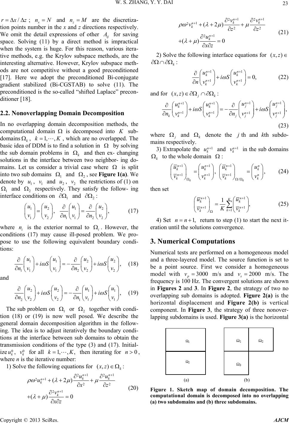

W. S. ZHANG, Y. Y. DAI 23

/rx z

; x and z are the discretiza-

tion points number in the x and z directions respectively.

We omit the detail expressions of other ij

nNnM

for saving

space. Solving (11) by a direct method is impractical

when the system is huge. For this reason, various itera-

tive methods, e.g. the Krylov subspace methods, are the

interesting alternative. However, Krylov subspace meth-

ods are not competitive without a good preconditioned

[17]. Here we adopt the preconditioned Bi-conjugate

gradient stabilized (Bi-CGSTAB) to solve (11). The

preconditioned is the so-called “shifted Laplace” precon-

ditioner [18].

2.2. Nonoverlapping Domain Decomposition

In no overlapping domain decomposition methods, the

computational domain  is decomposed into sub-

domainsk, , which are no overlapped. The

basic idea of DDM is to find a solution in by solving

the sub domain problems in k

1,k,K



and then ex- changing

solutions in the interface between two neighbor- ing do-

mains. Let us consider a trivial case where is split

into two sub domains 1

and 2

see Figure 1(a). We

denote by 1

u, 1 and 2

u, 2 restrictions of (1) on

 d 2

 pectively. They satisfy the follow- ing

interface conditions on 1

 d 2





vthe

resan :



























 



 



 (17)

where i is the exterior normal to i. However, the

conditions (17) may cause ill-posed problem. We pro-

pose to use the following equivalent boundary condi-

tions:

n

11 2



 





 



 









 iS







 (18)

and

22 1







(,)xz

22 1























(19)

The sub problem on 1 or 2 together with condi-

tion (18) or (19) is now well posed. We describe the

general domain decomposition algorithm in the follow-

ing. The idea is to adjust iteratively the boundary condi-

tions at the interface between sub domains to obtain the

transmission conditions of the type (3) and (17). Initial-

ize , for all then iterating for ,

where n is the iterative number:



1, ,k



v,0n

1) Solve the following equations for :



()

(2)



 





 















(20)

(2)

() 0











 





 



(21)

2) Solve the following in terface equations for (,)





 :





 







 

  (22)

and for (,)



:

11 11

nn jj

nn nn

iS iS





 

 





 

  



  

(23)

where



and k



denote the th and kth subdo-

mains respectively. j

3) Extrapolate the 1n



and in the sub domains

v



to the whole domain



111

, ,

nnn

kkk

nnn

kkk

uuu

vvv





 



 

 

(24)

then set









 



 

 

1





(25)

4) Set 1,nn



 return to step (1) to start the next it-

eration until the solutions convergence.

3. Numerical Computations

Numerical tests are performed on a homogeneous model

and a three-layered model. The source function is set to

be a point source. First we consider a homogeneous

model with 3000



m/s and m/s. The

frequency is 100 Hz. The convergent solutions are shown

in Figures 2 and 3. In Figure 2, the strategy of two no

overlapping sub domains is adopted. Figure 2(a) is the

horizontal displacement and Figure 2(b) is vertical

component. In Figure 3, the strategy of three nonover-

lapping subdomain s is used. Figu re 3(a) is the horizontal

2000

v

(a) (b)

Figure 1. Sketch map of domain decomposition. The

computational domain is decomposed into no overlapping

(a) two subdomains and (b) three subdomains.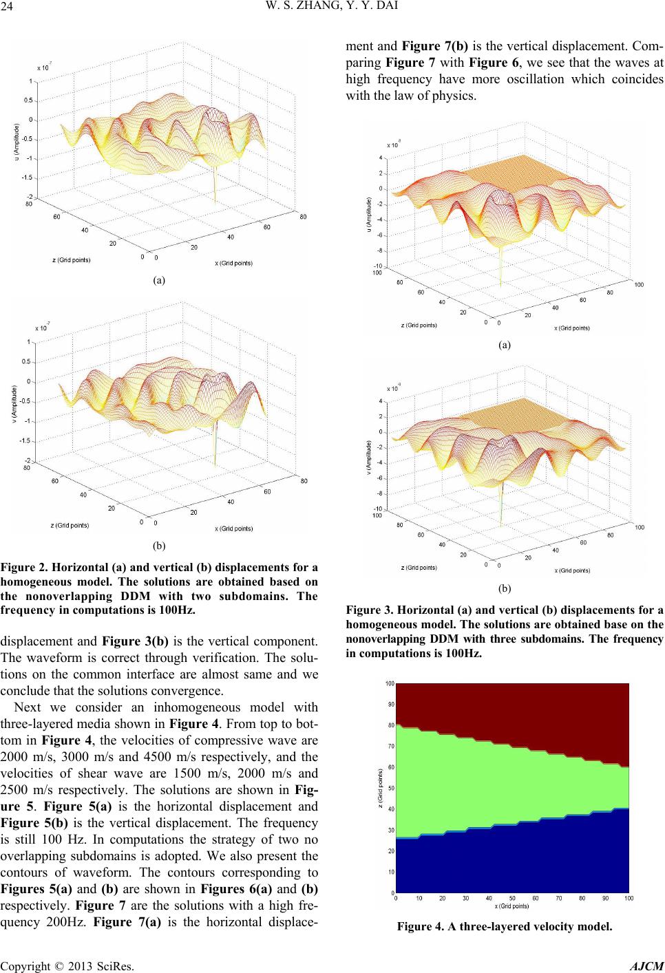

W. S. ZHANG, Y. Y. DAI

(a)

(b)

Figure 2. Horizontal (a) and vertical (b) displacements for a

homogeneous model. The solutions are obtained based on

the nonoverlapping DDM with two subdomains. The

freque ncy in computations is 100Hz.

displacement and Figure 3(b) is the vertical component.

The waveform is correct through verification. The solu-

tions on the common interface are almost same and we

conclude that the solutions convergence.

Next we consider an inhomogeneous model with

three-layered media shown in Figure 4. From top to bot-

tom in Figure 4, the velocities of compressive wave are

2000 m/s, 3000 m/s and 4500 m/s respectively, and the

velocities of shear wave are 1500 m/s, 2000 m/s and

2500 m/s respectively. The solutions are shown in Fig-

ure 5. Figure 5(a) is the horizontal displacement and

Figure 5(b) is the vertical displacement. The frequency

is still 100 Hz. In computations the strategy of two no

overlapping subdomains is adopted. We also present the

contours of waveform. The contours corresponding to

Figures 5(a) and (b) are shown in Figures 6(a) and (b)

respectively. Figure 7 are the solutions with a high fre-

quency 200Hz. Figure 7(a) is the horizontal displace-

ment and Figure 7(b) is the vertical displacement. Com-

paring Figure 7 with Figure 6, we see that the waves at

high frequency have more oscillation which coincides

with the law of physics.

(a)

(b)

Figure 3. Horizontal (a) and vertical (b) displacements for a

homogeneous model. The solutions are obtained base on the

nonoverlapping DDM with three subdomains. The frequency

in computations is 100Hz.

Figure 4. A three-layered velocity model.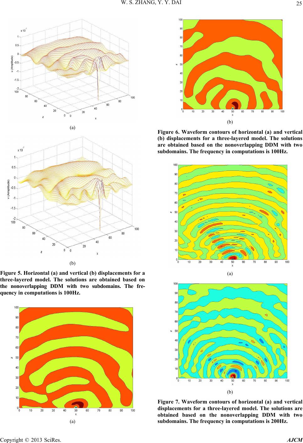

W. S. ZHANG, Y. Y. DAI 25

(a)

(b)

Figure 5. Horizontal (a) and vertical (b) displacements for a

three-layered model. The solutions are obtained based on

the nonoverlapping DDM with two subdomains. The fre-

quency in computations is 100Hz.

(a)

(b)

Figure 6. Waveform contours of horizontal (a) and vertical

(b) displacements for a three-layered model. The solutions

are obtained based on the nonoverlapping DDM with two

subdomains. The frequency in computations is 100Hz.

(a)

(b)

Figure 7. Waveform contours of horizontal (a) and vertical

displacements for a three-layered model. The solutions are

obtained based on the nonoverlapping DDM with two

subdomains. The frequency in computations is 200Hz.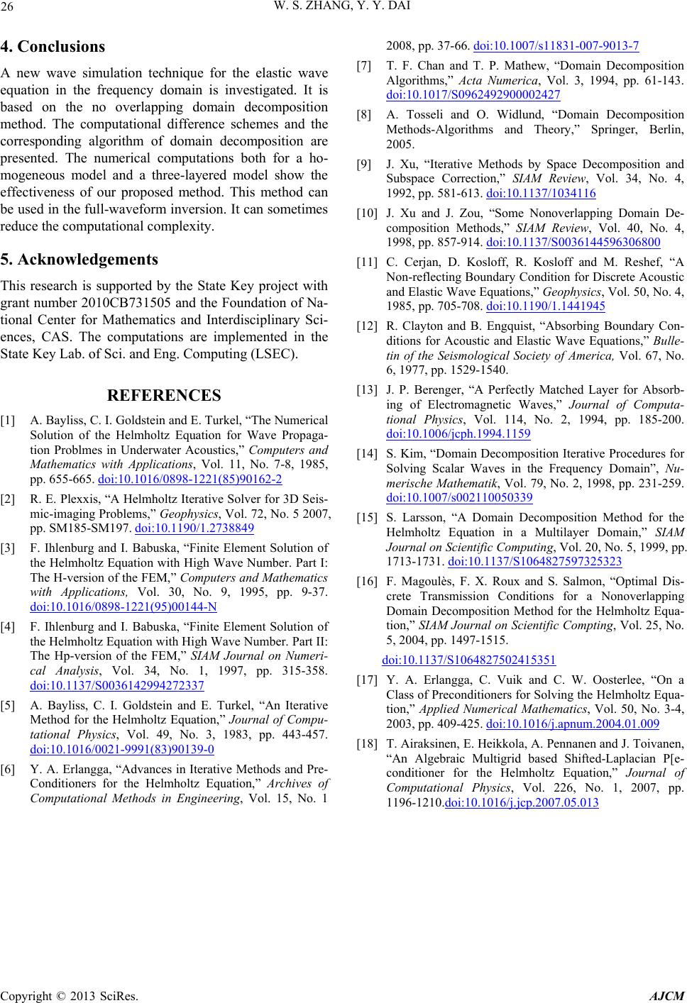

W. S. ZHANG, Y. Y. DAI

4. Conclusions

A new wave simulation technique for the elastic wave

equation in the frequency domain is investigated. It is

based on the no overlapping domain decomposition

method. The computational difference schemes and the

corresponding algorithm of domain decomposition are

presented. The numerical computations both for a ho-

mogeneous model and a three-layered model show the

effectiveness of our proposed method. This method can

be used in the full-waveform inversion. It can sometimes

reduce the computational complexity.

5. Acknowledgements

This research is supported by the State Key project with

grant number 2010 CB731505 and the Foundation of Na-

tional Center for Mathematics and Interdisciplinary Sci-

ences, CAS. The computations are implemented in the

State Key Lab. of Sci. and Eng. Computing (LSEC).

REFERENCES

[1] A. Bayliss, C. I. Goldstein and E. Turkel, “The Numerical

Solution of the Helmholtz Equation for Wave Propaga-

tion Problmes in Underwater Acoustics,” Computers and

Mathematics with Applications, Vol. 11, No. 7-8, 1985,

pp. 655-665. doi:10.1016/0898-1221(85)90162-2

[2] R. E. Plexxis, “A Helmholtz Iterative Solver for 3D Seis-

mic-imaging Problems,” Geophysics, Vol. 72, No. 5 2007,

pp. SM185-SM197. doi:10.1190/1.2738849

[3] F. Ihlenburg and I. Babuska, “Finite Element Solution of

the Helmholtz Equation with High Wave Number. Part I:

The H-version of the FE M,” Computers and Mathematics

with Applications, Vol. 30, No. 9, 1995, pp. 9-37.

doi:10.1016/0898-1221(95)00144-N

[4] F. Ihlenburg and I. Babuska, “Finite Element Solution of

the Helmholtz Equation with High Wave Number. Part II:

The Hp-version of the FEM,” SIAM Journal on Numeri-

cal Analysis, Vol. 34, No. 1, 1997, pp. 315-358.

doi:10.1137/S0036142994272337

[5] A. Bayliss, C. I. Goldstein and E. Turkel, “An Iterative

Method for the Helmholtz Equation,” Journal of Compu-

tational Physics, Vol. 49, No. 3, 1983, pp. 443-457.

doi:10.1016/0021-9991(83)90139-0

[6] Y. A. Erlangga, “Advances in Iterative Methods and Pre-

Conditioners for the Helmholtz Equation,” Archives of

Computational Methods in Engineering, Vol. 15, No. 1

2008, pp. 37-66. doi:10.1007/s11831-007-9013-7

[7] T. F. Chan and T. P. Mathew, “Domain Decomposition

Algorithms,” Acta Numerica, Vol. 3, 1994, pp. 61-143.

doi:10.1017/S0962492900002427

[8] A. Tosseli and O. Widlund, “Domain Decomposition

Methods-Algorithms and Theory,” Springer, Berlin,

2005.

[9] J. Xu, “Iterative Methods by Space Decomposition and

Subspace Correction,” SIAM Review, Vol. 34, No. 4,

1992, pp. 581-613. doi:10.1137/1034116

[10] J. Xu and J. Zou, “Some Nonoverlapping Domain De-

composition Methods,” SIAM Review, Vol. 40, No. 4,

1998, pp. 857-914. doi:10.1137/S0036144596306800

[11] C. Cerjan, D. Kosloff, R. Kosloff and M. Reshef, “A

Non-reflecting Boundary Condition for Discrete Acoustic

and Elastic Wave Equations,” Geophysics, Vol. 50, No. 4,

1985, pp. 705-708. doi:10.1190/1.1441945

[12] R. Clayton and B. Engquist, “Absorbing Boundary Con-

ditions for Acoustic and Elastic Wave Equations,” Bulle-

tin of the Seismological Society of America, Vol. 67, No.

6, 1977, pp. 1529-1540.

[13] J. P. Berenger, “A Perfectly Matched Layer for Absorb-

ing of Electromagnetic Waves,” Journal of Computa-

tional Physics, Vol. 114, No. 2, 1994, pp. 185-200.

doi:10.1006/jcph.1994.1159

[14] S. Kim, “Domain Decomposition Iterative Procedures for

Solving Scalar Waves in the Frequency Domain”, Nu-

merische Mathematik, Vol. 79, No. 2, 1998, pp. 231-259.

doi:10.1007/s002110050339

[15] S. Larsson, “A Domain Decomposition Method for the

Helmholtz Equation in a Multilayer Domain,” SIAM

Journal on Scientific Computing, Vol. 20, No. 5, 1999, pp.

1713-1731. doi:10.1137/S1064827597325323

[16] F. Magoulès, F. X. Roux and S. Salmon, “Optimal Dis-

crete Transmission Conditions for a Nonoverlapping

Domain Decomposition Method for the Helmholtz Equa-

tion,” SIAM Journal on Scientific Compting, Vol. 25, No.

5, 2004, pp. 1497-1515.

doi:10.1137/S1064827502415351

[17] Y. A. Erlangga, C. Vuik and C. W. Oosterlee, “On a

Class of Preconditioners for Solving the Helmholtz Equa-

tion,” Applied Numerical Mathematics, Vol. 50, No. 3-4,

2003, pp. 409-425. doi:10.1016/j.apnum.2004.01.009

[18] T. Airaksinen, E. Heikkola, A. Pennanen and J. Toivanen,

“An Algebraic Multigrid based Shifted-Laplacian P[e-

conditioner for the Helmholtz Equation,” Journal of

Computational Physics, Vol. 226, No. 1, 2007, pp.

1196-1210.doi:10.1016/j.jcp.2007.05.013