The Constrained Mean-Semivariance Portfolio Optimization Problem with the Support of a Novel Multiobjective Evolutionary Algorithm

doi:10.4236/jsea.2013.67B005

Paper Menu >>

Journal Menu >>

Journal of Software Engineering and Applications, 2013, 6, 22-29

doi:10.4236/jsea.2013.67B005 Published Online July 2013 (http://www.scirp.org/journal/jsea)

The Constrained Mean-Semivariance Portfolio

Optimization Problem with the Support of a Novel

Multiobjective Evolutionary Algorithm

K. Liagkouras, K. Metaxiotis

DSS Lab., Department of Informatics, University of Piraeus, Piraeus, Greece.

Email: [email protected], [email protected]

Received May, 2013

ABSTRACT

The paper addresses the constrained mean-semivariance portfolio optimization problem with the support of a novel

multi-objective evolutionary algorithm (n-MOEA). The use of semivariance as the risk quantification measure and the

real world constraints imposed to the model make the problem difficult to be solved with exact methods. Thanks to the

exploratory mechanism, n-MOEA concentrates the search effort where is needed more and provides a well formed effi-

cient frontier with the solutions spread across the whole frontier. We also provide evidence for the robustness of the

produced non-dominated solutions by carrying out, out-of-sample testing during both bull and bear market conditions

on FTSE-100.

Keywords: Multiobjective Optimization; Evolutionary Algorithms; Portfolio Optimization

1. Introduction

Portfolio optimization is the process of choosing the as-

sets and their proportions, so that it is attained the maxi-

mum profitability for the risk undertaken. MOEAs tech-

niques applied to the portfolio selection problem have

become increasingly popular relatively recen tly. Not only

because they provide a fast and reliable way of calculat-

ing computationally demanding financial models but also

why revolutionized the financial modeling research field

itself by developing innovative algorithmic approaches

for solving difficult financial problems that in many cas-

es cannot be solved with exact methods. Over the past

years researchers developed several approaches for the

solution of the portfolio optimization problem with the

use of MOEAs. Most of the early work on MOEAs

adopts the unconstrained Markowitz Mean – Variance

(MV) model [2, 4]. Obvio u sl y , the p rac t i cal usef ul ness of

such a model is limited to acad emic purposes an d cannot

address the complexity and multiple real world con-

straints faced by portfolio managers. More recent studies,

incorporate a number of constrain ts into the optimization

model, but do not examine how these constraints affect

the evolutionary search process and the efficient frontier

formulation. Additionally, still the majority o f the studies

use variance [3] for the quantification of portfolio risk

although it’s well known undesirable mathematical

properties [1].

Our paper proposes a bi-objective return semivariance

portfolio optimization model that incorporates a number

of real world constraints such as cardinality constraints,

floor and ceiling constraints, non-negativity constraint

and budget constraint and analyzes their effects on the

efficient frontier formulation. Finally, we provide em-

pirical evidence for the robustness of the proposed

methodology by performing, out-of-sample experiments

during both bull and bear market conditions on FTSE-

100.

The paper is organized as follows. Section 2 provides

a formal introduction of the proposed multi-objective

portfolio optimization model and the various constraints

applied. Section 3 provides an analytical description of

the proposed MOEA model, focusing especially on the

applied techniques for the efficient exploration of the

search space. Finally, section 4 evaluates the robustness

of the proposed algorithm by carrying out a number of

out-of-sample tests during both bull and bear market

conditions.

2. Problem Definition

The Portfolio optimization problem seeks to optimize

two conflicting objectives, portfolio return and risk (Ta-

ble 1) subject to a set of constraints. In multi-objective

optimization, and particularly when the objectives are

conflicting, there is not a single solution that can opti-

The Constrained Mean-Semivariance Portfolio Optimization Problem with the Support of a

Novel Multiobjective Evolutionary Algorithm 23

mize all objectives simultaneously. Thus, in reality we

are trying to find good compromises or “trade-offs” be-

tween the different objectives. This “trade-off” between

the different objectives was expressed for first time by

Francis Edgeworth and generalized by Vilfredo Pareto.

Nowadays, is known as Pareto optimality. Let



be the

search space. Consider 2 objective functions 12

where and . :

f 

Table 1. The Portfolio Optimization Problem

Optimize

()((), ())

wfwfw

Maximize portfolio return 11

() m

fw wr





Minimize portfolio risk 211

() mm

ijij

fx wwss







where:

Decision variables 1 subject to ( ,..,)

www



w

and m = 100 equal to the number of stocks in FTSE-100.

Rate of return of assets .

,..,

rr r



is the correlation between asset i and j and





ss ,

.

ji represent the semi-standard deviation of stocks

returns i and j respectively. The formula is

1()

ii tR

SSV rT

n

 

,

where i represents the semivariance of security i.

represents the target return, equal to zero in this occasion

and tR

the difference between realized return and

target return.

rT

2.1. Constraints to the Problem

Budget constraint or summation constraint





requires all portfolios to have non-negative weights

(i) that sum to 1. The non-negativity

constraint indirectly implies that short selling is not al-

lowed.

10  w1,..,im

Floor and ceiling constraints .

Where ai = the minimum weighting that can be held of

asset i (i = 1, …, n ), bi = the maximum weighting that

can be held of asset i(i = 1, …, n ) and

,1,2,...,

iii

awb n

ab

1,2,...,n

Cardinality constraint , where:

min max







Cmin = the minimum number of assets that a portfolio

can hold

Cmax = the maximum number of assets that a portfolio

can hold

1, 0

0, 0

qforw













2.2. Pareto Optimality Definitions

We make use of Pareto optimality framework in order to

determine the solutions in this multi-objective optimiza-

tion problem. In particular we use the following defini-

tions:

Definition 1 (Pareto dominance)

Consider a maximization problem. Let x, y be two de-

cision vectors (solutions) from Ω. Solution x dominate y

(also written as x > y) if and only if the following condi-

tions are fulfilled: (i) The solution x is no worse than y in

all objectives ii (ii) The solu-

tion x is strictly better than y in at least one objective

nyfxf ,...,2,1),()(

}:( )()

fxfy{1,2,...,jn



. If any of the above con-

ditions is violated the solution x does not dominate the

solution y.

Definition 2 (Global Pareto-Optimal set)

The non-dominated set of the entire feasible search

space Ω is the global Pareto-optimal set.

Definition 3 (Local Pareto-Optimal set)

Let



S be a subset of the search space. All solu-

tions which are not dominated by any vector of S are

called non-dominated with respect to S. Solutions that

are non-dominated with respect to S, are called

local Pareto solutions or local Pareto regions.

S

Definition 4 (Strong dominance)

A solution x strongly dominates a solution y, x > y, if

solution x is strictly better than solution y in all m objec-

tives.

Definition 5 (Weak dominance)

A solution x weakly dominates y, if ( )(),1,2,...,

xfy n

and there is no x



 such that ()(), 1,2,...,

xfyin





Definition 6 (Non dominated solutions)

A solution x is called non-dominated if x is either a

strong non-dominated or a weak non-dominated.

Figure 1 we provide a schematic illustration of the

dominance in a bi-objective optimization (portfolio re-

turn and risk), where a higher value is better for f1(w) =

“Return objective function” and a lower value is better

for f2(w) = “Risk objective function”

In this example solution A1 strongly dominates solu-

tion A2, A3 and B since th e f1(w) and f2(w) of solution A1

are strictly better than the f1(w) and f2(w) of so lution A2 ,

A3 and B respectively. Solution A and C are weakly

dominated by solution A1 where the value of one of the

objectives functions of the dominated solution is equal to

the corresponding value of solution A1.

3. The Proposed Methodology

The Constrained Mean-Semivariance Portfolio Optimization Problem with the Support of a

Novel Multiobjective Evolutionary Algorithm

This section is dedicated to the presentation of the pro-

posed MOEA. The n-MOEA is summarized in the fol-

lowing steps.

Algorithm_n-MOEA()

Figure 1. Pareto optimization in mean-risk portfolio opti-

mization problem.

1) INITIALIZATION of the population

2) WHILE termination criterion not fulfilled

3) EVALUATE each portfolio of the population using

Pareto Optimality

4) ARCHIVE add th e Local non-dominated por tfolios

into the archive

5) EVALUATE_ARCHIVE according to Pareto Op-

timality conditions

5a. DOMINATED_SOLUTIONS removed from

ARCHIVE

5b. NON_DOMINATED remain into the ARCHIVE

as Global Non-dominated so lutions

6) REPRODUCTION_FITNESS assign reproduction

fitness to the Global non-dominated portfolios according

to the Euclidian distance between them.

7) CREATE_NEW_POPULATION new population

is created probabilistically from the Global non-domi-

nated solutions in the ARCHIVE according to the fitness

assigned to each portfolio.

8) MUTUTION operation applied to the new popula-

tion to variate the portfolios

9) CROSSOVER operation applied to the new popu-

lation to preserve population diversity.

10) GO TO step 2

Below we provide analytical description of the key

elements of the proposed algorithm.

3.1. Reproduction Fitness Assignment

As soon as, we identify the Global non-dominated solu-

tions, we arrange them into the Cartesian system. Thus,

for any solution into the system we know the two neigh-

bor solutions (portfolios). Please, note that the most left-

ward and rightward points (E and D in this occasion)

have one neighbor solution. Next, we calculate the Eu-

clidian distance for each Global non-dominated solution

(portfolio) in the Archive (see Figure 2).

where: 22

()(

ABA A

return risk

dreturn



)

risk

((

))

AC A

AC return returnriskrisk

d

Generally, the distance between two points x = (x1,…,

xn) and y = (y1,…, yn) in Euclidean n-space is given by:

112 2

(,) ...

()()(

()

dxy 2

)

yxy xy









We assign reproduction fitness to each Global non-

dominated solution. The reproduction fitness points sum

up to 1% or 100%. The reproduction fitness is assigned

according to the Euclidian distance of the solution from

its neighbor solutions. Thus, the higher the Euclidean

distance of the solution, the higher gets the assigned re-

production fitness. The reproduction fitness assigned to

the Global non-dominated Archive solutions will guide

the exploratory process.

3.2. Generation of New Population

Then, probabilistically are selected the solutions (portfo-

lios) that will be included in the new population. Obvi-

ously, the higher fitness solutions have more chances to

be picked up. Depending on the size of population and

the number of Global non-dominated solutions in the

Archive, many copies of Solution A may be reproduced

in the new population. For example if the population size

is 50 and the non-dominated solutions in the Ar chive are

10, and assuming that solution A had much higher fitness

(see Figure 3) than any other solution in the Archive,

then we would expect solution A to be reproduced more

Figure 2. Calculation of the Euclidian distance between the

Global non-dominated solutions for the assignment of re-

production fitness.

The Constrained Mean-Semivariance Portfolio Optimization Problem with the Support of a

Novel Multiobjective Evolutionary Algorithm

Figure 3. Global non-dominated solution A is assigned a

higher reproduction fitness, due to its higher Euclidian dis-

tance from the rest non-dominated solutions.

than 5 times (average reproduction) in the new popula-

tion due to the higher reproduction fitness.

3.3. The Mutation Mechanism

The number of mutants is determined by the portfolio

size and the mutation rate. For determining which stocks

will exist the portfolio is calculated the Inverse Fitness.

The Inverse Fitness is calculated as follows:

Inverse Fitness = Maximum Stock Fitness

– Stock Fitness

where: Maximum Stock Fitness: The stock with the high-

est fitness among the stocks on FTSE-100 and Stock Fit-

ness: The fitness of each individual stock that is included

in the portfolio.

That means that the highest fitness stock of FTSE-100

has an Inverse Fitness of zero. As soon as we calculate

the portfolio’s Inverse Fitness, we probabilistically select

the stocks to exit the portfolio. Obviously, the highest

fitness stock will not exit the portfolio as has an Inverse

Fitness of zero. Stocks with higher inverse fitness and

thus lower fitness are more probable to be removed from

the portfolio. This is an elitism mechanism that gives

probabilistic advantage to the higher fitness stocks to

remain into the portfolio.

Having decided which stocks will exit the portfolio,

and then we have to determine which stocks will enter

the portfolio as mutants. In this case all the stocks of the

index are taken into account, according to their fitness.

Again, cardinality constraints and lower and upper b ou nd s

are taken into account during this process. Taking stocks’

fitness into account means that stocks with higher fitness

are more probable to enter the portfolio as mutants.

3.4. The Crossover Mechanism

At this stage, the population already has been variated

through the mutation process. In order to maintain diver-

sity in the population and avoid convergence to a single

solution we make use of the crossover mechanism. The

crossover between the various solutions (portfolios) is

random, but within the maximum and minimum cross-

over rates that we have specified at an earlier stage. For

example if we specify maximum crossover rate = 90%

and minimum = 70%, that means that randomly will be

selected a crossover rate within these limits let’s say 80%.

A crossover rate 80% simply means that 80% of portfolio

A will be crossover with 20% of portfolio B and 20% of

portfolio A will be crossover with 80% of portfolio B.

Please note that the pairs to be crossover are selected

randomly.

3.5. Efficient Frontier Formulation

Next, we present the process of efficient frontier formu-

lation by quoting experimental results based on historical

data of FTSE-100. For the first experiment, as a training

set we use 63 daily historical observations of FTSE-100

from 30-Nov-2011 till 29-Feb-2012. The configuration

of the n-MOEA for this experiment is: population size 70,

maximum number of generations 200, floor constraint

5%, ceiling constraint 31%, Cardinality constraint 20

stocks, crossover rate between 70% and 90% and muta-

tion rate 20%. Below, we provide two figures with the

Efficient Frontier formulation at different stages of the

algorithm execution.

Figure 4 displays the exploratory process of n-MOEA.

It is evident even from Figure 4(a) at generation 50 that

the algorithm pusses the exploratory process towards the

left and upward corn er of the figure where the most effi-

cient solutions reside i.e. solutions that command higher

return and lower risk. At generation 200 as it is evident

from Figure 4(b) the region surrounding the efficient

frontier has been turned solid grey, meaning that given

the constraints imposed has been exhausted the possibil-

ity to move the efficient frontier further towards the left

and upward corner of the figure.

4. Robustness of n-MOEA

In relevant literature there are different views about ro-

bustness. Some scholars define robustness as the consis-

tency of results between different runs of the algorithm;

others define robustness as the insensitivity of solution to

small changes in the decision variables. We will examine

the robustness of the proposed algorithm from a practical

point of view. Specifically, we will test the robustness of

the obtained solutions in out-of-sample environments.

For this experiment we use a training set of 63 daily his-

torical observations of FTSE-100 from 30-Nov-2011 till

29-Feb-2012. The configuration of the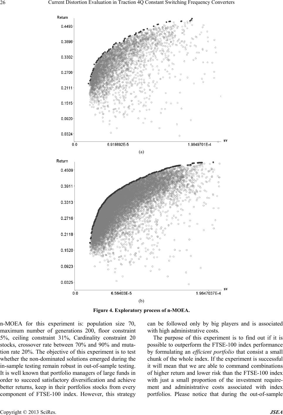

Current Distortion Evaluation in Traction 4Q Constant Switching Frequency Converters

(a)

(b)

Figure 4. Exploratory process of n-MOEA.

n-MOEA for this experiment is: population size 70,

maximum number of generations 200, floor constraint

5%, ceiling constraint 31%, Cardinality constraint 20

stocks, crossover rate between 70% and 90% and muta-

tion rate 20%. The objective of this experiment is to test

whether the non-dominated solutions emerged during the

in-sample testing remain robust in out-of-sample testing.

It is well known that portfolio managers of large funds in

order to succeed satisfactory diversification and achieve

better returns, keep in their portfolios stocks from every

component of FTSE-100 index. However, this strategy

can be followed only by big players and is associated

with high administrative costs.

The purpose of this experiment is to find out if it is

possible to outperform the FTSE-100 index performance

by formulating an efficient portfolio that consist a small

chunk of the whole index. If the experiment is successful

it will mean that we are able to command combinations

of higher return and lower risk than the FTSE-100 index

with just a small proportion of the investment require-

ment and administrative costs associated with index

portfolios. Please notice that during the out-of-sample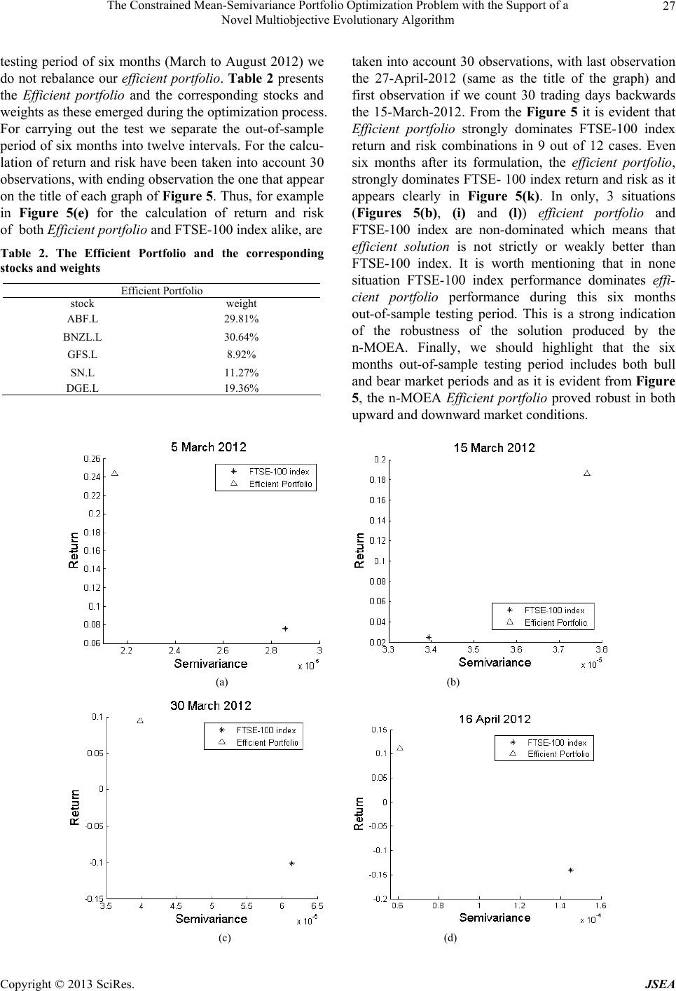

The Constrained Mean-Semivariance Portfolio Optimization Problem with the Support of a

Novel Multiobjective Evolutionary Algorithm 27

testing period of six months (March to August 2012) we

do not rebalance our efficient portfolio. Table 2 presents

the Efficient portfolio and the corresponding stocks and

weights as these emerged during the optimization process.

For carrying out the test we separate the out-of-sample

period of six months into twelve intervals. For the calcu-

lation of return and risk have been taken into account 30

observations, with ending observation the one that appear

on the title of each graph of Figure 5. Thus, for example

in Figure 5(e) for the calculation of return and risk

of both Efficient portfolio and FTSE-100 index alike, are

Table 2. The Efficient Portfolio and the corresponding

stocks and weights

Efficient Portfolio

stock weight

ABF.L 29.81%

BNZL.L 30.64%

GFS.L 8.92%

SN.L 11.27%

DGE.L 19.36%

taken into account 30 observations, with last observation

the 27-April-2012 (same as the title of the graph) and

first observation if we count 30 trading days backwards

the 15-March-2012. From the Figure 5 it is evident that

Efficient portfolio strongly dominates FTSE-100 index

return and risk combinations in 9 out of 12 cases. Even

six months after its formulation, the efficient portfolio,

strongly dominates FTSE- 100 index return and risk as it

appears clearly in Figure 5(k). In only, 3 situations

(Figures 5(b), (i) and (l)) efficient portfolio and

FTSE-100 index are non-dominated which means that

efficient solution is not strictly or weakly better than

FTSE-100 index. It is worth mentioning that in none

situation FTSE-100 index performance dominates effi-

cient portfolio performance during this six months

out-of-sample testing period. This is a strong indication

of the robustness of the solution produced by the

n-MOEA. Finally, we should highlight that the six

months out-of-sample testing period includes both bull

and bear market periods and as it is evident from Figure

5, the n-MOEA Efficient portfolio proved robust in both

upward and downward market conditions.

(a) (b)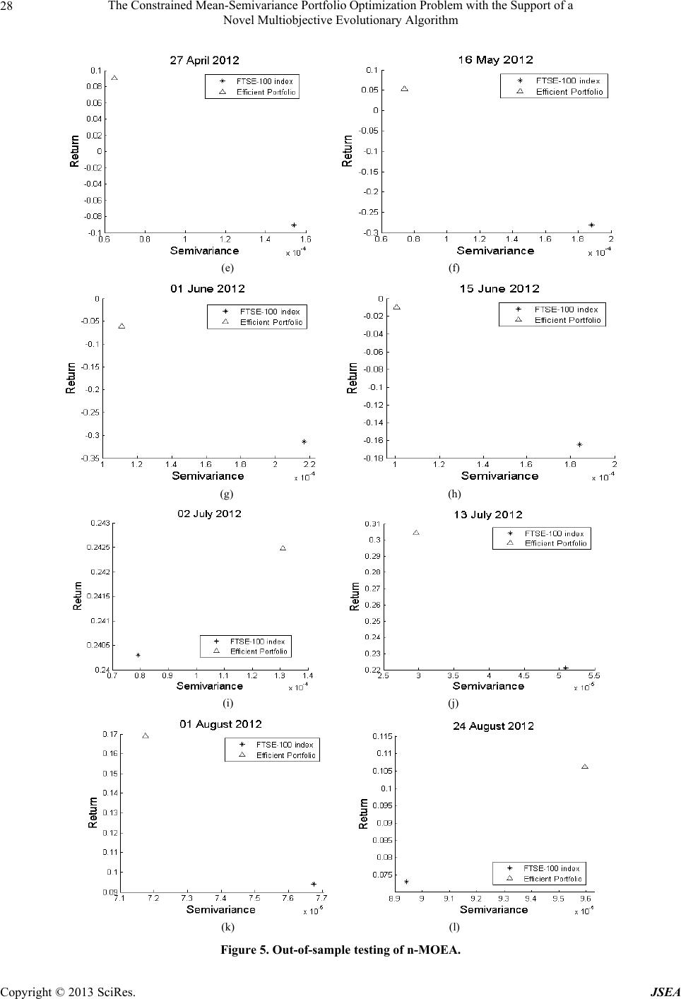

The Constrained Mean-Semivariance Portfolio Optimization Problem with the Support of a

Novel Multiobjective Evolutionary Algorithm

(e) (f)

(g) (h)

(i) (j)

(k) (l)

Figure 5. Out-of-sample testing of n-MOEA.

The Constrained Mean-Semivariance Portfolio Optimization Problem with the Support of a

Novel Multiobjective Evolutionary Algorithm

5. Conclusions

In this paper, we have proposed a novel MOEA for the

solution of the constrained mean-semivariance portfolio

optimization problem. The algorithm can handle suc-

cessfully downside risk measures like semivariance and

real world constraints and formulate well spread frontiers

thanks to an elitism mechanism applied in the mutation

process that give a reproduction advantage to the higher

fitness stocks, and an exploratory mechanism that uses

the notion that good solutions are more probable to be

found near other non-dominated solutions. At the same

time another mechanism calculates the Euclidian dis-

tance between the various non-dominated solutions in

order to assign reproduction fitness. That way, we safe-

guard that the exploratory effort is concentrated where is

needed more and the solutions are spread across the en-

tire frontier. Also, the crossover process enhances the

population diversity, by combining randomly two

non-dominated solutions to produce two new off-springs.

The robustness of the proposed algorithm is verified for

short and mid-term by carrying out a number of

out-of-sample tests during both bull and bear market

conditions on FTSE-100.

REFERENCES

[1] P. Artzner, F. Delbaen, J. Eber and D. Heath, “Coherent

measures of risk. Mathematical Finance,”Mathematical

Finance, Vol. 9, No.3, pp.203–228.

doi:10.1111/1467-9965.00068

[2] H. M. Markowitz, “Foundations of Portfolio Theory,”

Journal of Finance, Vol.46, No. 2, 1991, pp.469-477.

doi:10.1111/j.1540-6261.1991.tb02669.x

[3] K. Metaxiotis and K. Liagkouras, “Multiobjective Evolu-

tionary Algorithms for Portfolio Management: A com-

prehensive Literature Review,” Expert Systems with Ap-

plications 39, Vol.39, No. 14, 2012, pp.11685–11698.

doi:10.1016/j.eswa.2012.04.053

[4] F. Pasiouras, S. Tanna and C. Zopounidis, “The Impact of

Banking Regulations on Bank’s Cost and Profit Effi-

ciency: Cross country Evidence,” International Review of

Financial Analysis, Vol. 18, No. 5, 2009, 294 - 302.

doi:10.1016/j.irfa.2009.07.003