Compensation of Finite Bandwidth Effect by Using an Optimal Filter in Photoacoustic Imaging

doi:10.4236/eng.2013.510B006

Paper Menu >>

Journal Menu >>

Engineering, 2013, 5, 27-31

http://dx.doi.org/10.4236/eng.2013.510B006 Published Online October 2013 (http://www.scirp.org/journal/eng)

Compensation of Finite Bandwidth Effect by Using an

Optimal Filter in Photoacoustic Imaging*

Chen Zhang, Yan Zhang, Yuanyuan Wang

Department of Electronic Engineering, Fudan University, Shanghai, China

Email: [email protected], [email protected]

Received September 2012

ABSTRACT

Most existing reconstruction algorithms for photoacoustic imaging (PAI) assume that transducers used to receive ultra-

sound signals have infinite bandwidth. When transducers with finite bandwidth are used, this assumption may result in

reduction of the imaging contrast and distortions of reconstructed images. In this paper, we propo s e a novel method to

compensate the finite bandwidth effect in PAI by using an optimal filter in the Fourier domain. Simulation results

demonstrate that the use of this method can improve the contrast of the reconstruc ted images with finite-bandwidth ul-

trasound transducers.

Keywords: Photoacoustic Tomography; Finite Bandwidth Effect; Optimal Filter

1. Introduction

Photoacoustic imaging (PAI) is a promising medical im-

aging modality that has great potential for a wide ra nge

of clinical imaging applications [1,2]. PAI is a hybrid

imaging method that combines the high contrast of opti-

cal imaging and the high spatial resolution of ultrasonic

imaging. Due to its noninvasive nature, it is a technique

which is harmless for the human body [2].

In PAI, pulsed laser energy is delivered to an object

and the thermoacoustic effect will result in the generation

of the ultr asound wav e. Ultrasound signals are t hen de-

tected by the scanning ultrasound transducers. With these

received signals, an image reconstruc tion algorithm is

used to reconstruct the image of an object’s optical ab-

sorption distribution.

A variety of research has been done on the f ield of

image reconstr uction algorithms [3-10]. Most of these

algorithms are based on th e assumption that infinite-

bandwidth transducers are employed to receive ultra-

sound signals. Without incorporating characteristics of

ultrasound transducers in the imaging reconstruction

model, the resolution and the contrast of reconstructed

images will be significantly degraded. Several imaging

models have been established to incorporate physical

characteristics of ultrasound transducers [11,12]. How-

ever, none of them takes the finite bandwidth effect of

ultrasound tr ansd uc e r s into account.

In this paper, we propose a novel image reconstruction

algorithm that incorporates the finite ba ndwidth ch arac-

teristics of ultrasound tr ansducers. An optimal filter is

designed to deconvolve the transducer’s impulse re-

sponse of the finite bandwidth at each imaging point.

Through the numerical simulation, the proposed algo-

rithm is compared to those recons truction algorithms

assuming finite-bandwidth ultrasound transducers.

2. Theory and Method

2.1. Basic Principles of PAI

In this study, we intend to solve the problem with 2D

circular-scanning PAI mode. In this mode, a short pulse

is used to illuminate the imaging object from the top, and

an ultrasoun d transducer is circularly sc anned a rou nd the

object to record the ultr a s ound data. The relation between

the optical absorption distribution and the gen erated ul-

trasonic waves can be deduced as [3]:

1 (,)()

(,) ()

p tIt

pt A

∂∂

∇−=− ∂

∂

, (1)

where c is the speed of sound,

is the volume thermal

expansion coefficient and Cp is the specific heat. A(r) is

the unknown absorption distribution and I(t) is the illu-

mination function. A solution to this equation can be

obtained by the use of Green’s function. In the case of

illumination with a short pulse, p(r, t) can be deduced as:

( ')

( ,)'

4ct

pt d

Ct t

−=

∂

=∂∫∫rr



(2)

Equation (2) represent s an idealized imaging model for

*Natural Science Foundation of China (

No. 61271071 and No.

11228411) and Specialized Research Fund forthe Doctoral

Program of

Higher Edu cation of China (No. 201 1 0 071110017).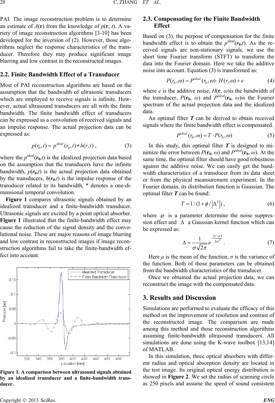

C. ZHANG ET AL.

PAI. The image reconstruction problem is to determine

an estimate of A(r) from the know ledge of p(r, t). A va-

riety of image reconstruction algorithms [3-10] ha s been

developed for the inversion of (2). However, those algo-

rithms neglect the response characteristics of the trans-

ducer. Therefore they may produce significant image

blurring and low contrast in the reconstructed images.

2.2. Finite Bandwidth Effect of a Transducer

Most of PAI reconstruction algorithms are based on the

assumption that the bandwidth of ultrasonic transducers

which are employed to receive signals is infinite. How-

ever, actual ultrasound transducer s are all with the finite

bandwidth. The finite bandwidth effect of transducers

can be expressed as a convolution of received signals and

an impulse respon se. The actual projection data can be

expressed as:

( ,)( ,)(,)

ideal

prtprt hrt= ∗

, (3)

where the pideal(r0,t) is the idealized projection data based

on the assumption that the transducers have the infinite

bandwidth, p(r0,t) is the actual projection data obtained

by the transducers, h(r0,t) is the impulse response of the

transducer related to its bandwidth, * denotes a one-di-

mensional temporal convolution.

Figure 1 compares ultrasonic signals obtained by an

idealized transducer and a finite-bandwidth transducer.

Ultrasonic signals are excited by a point optical absorber.

Figure 1 illustrated that the finite-bandwidth effect may

cause the reduction of the signal density and the convo-

lutional noise. These are major reasons of image blurr ing

and low contrast in reconstructed images if image recon-

struction algorithms fail to take the finite-bandwidth ef-

fect into account.

Figure 1. A comparison between ultrasou nd signals obtaine d

by an idealized transducer and a finite-bandwidth trans-

ducer.

2.3. Compensating for the Finite Bandwidth

Effect

Based on (3), the purpos e of compensation for the finite

bandwidth effect is to obtain the pideal(r0,t). As the re-

ceived signals are non-stationary signals, we use the

short time Fourier transform (STFT) to transform the

data into the Fourier domain. Here we take the additive

noise into account. Equation (3) is transformed as:

(,)(,) (,)

ideal

PrP rHre

ω ωω

= ⋅+

(4)

where e is the additive noise, H(r, ω)is the bandwidth of

the transducer, P(r0, ω) and Pideal(r0, ω)is the Fourier

spectrum of the actual projection data and the idealized

data.

An optimal filter T can be derived to obtain received

signals wher e th e finite bandwidth effect is compensated.

(,) (,)

ideal

PrTPr

ωω

= ⋅

(5)

In this study, this optimal filter T is designed to mi-

nimize the error between P(r0, ω) and Pideal(r0, ω). At the

same time, th e optimal filter should have good robustness

against the additive noise. We can easily get the band-

width characteristics of a transducer from its data sheet

or from the physical meansurement experiment. In the

Fourier domain, its distribution function is Gaussian. The

optimal filter T can be found:

1 /(1/)T

= +∆

, (6)

where

is a parameter determine the noise suppres-

sion effect and

∆

a Gaussian kernel function which can

be expressed as:

()

σπ

−

∆=

. (7)

Here μ is the mean of the function, σ is the variance of

the function. Both of those parameters can be obtained

from the bandwidth characteristics of the transducer.

Once we obtained the actual projection data, we can

reconstruct the image with the compensated data.

3. Results and Discussion

Simulations are performed to ev alu ate the efficacy of this

method on the improvement of resolution and contrast of

the reconstructed image. The comparison are made

among this method and those reconstruction algorithms

assuming finite-bandwidth ultrasound transducers. All

simulations are done using the K-wave toolbox [13,14]

of MATLAB.

In this simulation, three optical absorbers with differ-

ent radius and optical absorption density are located in

the test image. Its original optical energy distribution is

showed in Figure 2. We set the radius of scanning circle

as 250 pixels and assume the speed of sound consistent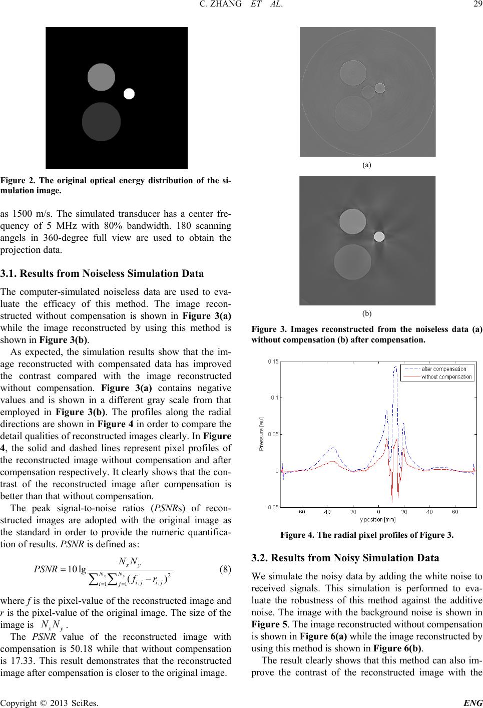

C. ZHANG ET AL.

Figure 2. The original optical energy distribution of the si-

mulation image.

as 1500 m/s. The simulated transducer has a center fre-

quency of 5 MHz with 80% bandwidth. 180 scanning

angels in 360-degree full view are used to obtain the

projection data.

3.1. Results from Noiseless Simulation Data

The computer-simulated noiseless data are used to eva-

luate the efficacy of this method. The image recon-

structed without compensation is shown in Figure 3(a)

while the image reconstructed by using this method is

shown in Figure 3(b).

As expected, the simulation results show that the im-

age reconstructed with compensated data has improved

the contrast compared with the image reconstructed

without compensation. Figure 3(a) contains negative

values and is shown in a different gray scale from that

employed in Figure 3(b). The profiles along the radial

directions are shown in Figure 4 in order to compare the

detail qualities of reconstructed images clearly. In Figure

4, the solid and dashed lines represent pixel profiles of

the reconstructed image without compensation and after

compensation respectively. It clearly shows that the con-

trast of the reconstructed image after compensation is

better than that without compensation.

The peak signal-to-noise ratios (PSNRs) of recon-

structed images are adop ted with the original image as

the standard in order to provide the numeric quantifica-

tion of results. PSNR is defined as:

10lg ()

ij ij

PSNR fr

= =

=−

∑∑

(8)

where f is the pixel-value of the reconstructed image and

r is the pixel-value of the original image. The size of the

image is

The PSN R value of the reconstructed image with

compensation is 50.18 while tha t without compensation

is 17.33. This result demonstrates that the reconstructed

image after compensation is closer to the original image.

(a)

(b)

Figure 3. Images reconstructed from the noiseless data (a)

without compensation ( b) after co m pe nsation.

Figure 4. The radial pixel profiles of Figure 3.

3.2. Results from Noisy Simulation Data

We simulate the noisy data by adding the white noise to

received signals. This simulation is performed to eva-

luate the robustness of this method against the additive

noise. The image with the back ground noise is shown in

Figure 5. The image reconstructed without compensation

is shown in Figure 6(a) while the image reconstructed by

using this method is shown in Figure 6(b).

The result clearly shows that this method can also im-

prove the contrast of the reconstructed image with the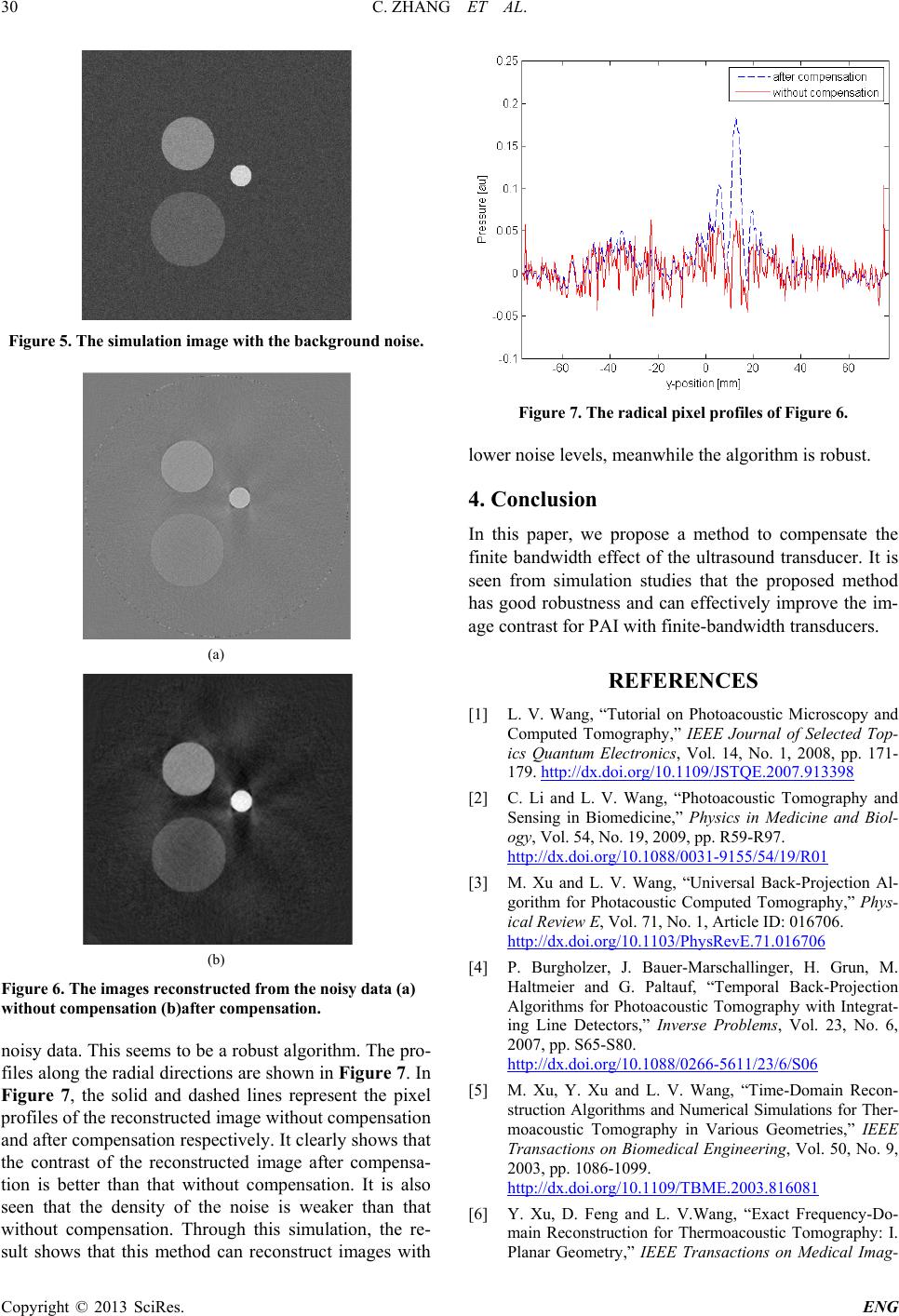

C. ZHANG ET AL.

Figure 5. The simulation image with the background noise .

(a)

(b)

Figure 6. The images reconstructed from the noisy data (a)

without compensation (b)after co m pe nsation.

noisy data. This seems to be a robust algorithm. The pro-

files along the radial directions are shown in Figure 7. In

Figure 7, the solid and dashed lines represent the pixel

profiles of the reconstructed image without compensation

and after compensation respectively. It clearly shows that

the contrast of the reconstructed image after compensa-

tion is better than that without compensation. It is also

seen that the density of the noise is weaker than that

without compensation. Through this simulation, the re-

sult shows that this method can reconstruct images with

Figure 7. The radical pixel profiles of Figure 6.

lower noise levels, meanwhile the algorithm is robust.

4. Conclusion

In this paper, we propose a method to compensate the

finite bandwidth effect of the ultrasou nd transducer. It is

seen from simulation studies that the proposed method

has good robustn es s and can effectively improve the im-

age contrast for PAI with finite-bandwidth transducers.

REFERENCES

[1] L. V. Wang, “Tutorial on Photoacoustic Microscopy and

Computed Tomography,” I EEE Journal of Selected Top-

ics Quantum Electronics, Vol. 14, No. 1, 2008, pp. 171-

179. http://dx.doi.org/10.1109/JSTQE.2007.913398

[2] C. Li and L. V. Wang, “Photoacoustic Tomography and

Sensing in Biomedicine,” Physics in Medicine and Biol-

ogy, Vol. 54, No. 19, 2009, pp. R59-R97.

http://dx.doi.org/10.1088/0031-9155/54/19/R01

[3] M. Xu and L. V. Wang, “Universal Back-Projection Al-

gorithm for Photacoustic Computed Tomography,” Phys-

ical Review E, Vol. 71, No. 1, Article ID: 016706.

http://dx.doi.org/10.1103/PhysRevE.71.016706

[4] P. Burgholzer, J. Bauer-Marschallinger, H. Grun, M.

Haltmeier and G. Paltauf, “Temporal Back-Projection

Algorithms for Photoacoustic Tomography with Integrat-

ing Line Det ectors,” Inverse Problems, Vol. 23, No. 6,

2007, pp. S65-S80.

http://dx.doi.org/10.1088/0266-5611/23/6/S06

[5] M. Xu, Y. Xu and L. V. Wang, “Time-Doma in Recon-

struction Algorithms and Numerical Simulations for Ther-

moacoustic Tomography in Various Geometries,” IEEE

Transactions on Biomedical Engineering, Vol. 50, No. 9,

2003, pp. 1086-1099.

http://dx.doi.org/10.1109/TBME.2003.816081

[6] Y. Xu, D. Feng and L. V.Wang, “Exact Frequency-Do-

main Reconstruction for Thermoacoustic Tomography: I.

Planar Geometry,” IEEE Transactions on Medical Imag-

C. ZHANG ET AL.

ing, Vol. 21, No. 7, 2002, pp. 823-828.

http://dx.doi.org/10.1109/TMI.2002.801172

[7] L. A. Kunyansky, “Explicit Inversion Formulae for the

Spherical Mean Radon Transform,” Inverse Proble ms,

Vol. 23, 2007, pp. 373-383.

http://dx.doi.org/10.1088/0266-5611/23/1/021

[8] M. A. Anastasio, J. Zhang, X. Pan, Y. Zou, G. Keng and

L. V. Wang, “Half-Time Image Reconstruction in Ther-

moacoustic Tomography,” IEEE Transactions on Medi-

cal Imaging, Vol. 24, No. 2, 2005, pp. 199-210.

http://dx.doi.org/10.1109/TMI.2004.839682

[9] P. Ephrat, L. Keenliside, A. Seabrook, F. S. Prato and J. J.

L. Carson, “Three-Dimensional Photoacoustic Imaging

by Sparse-Arra y Detection and Iterative Image Recon-

struction,” Journal of Biomedical Optics, Vol. 13, No. 5,

2008. http://dx.doi.org/10.1121/1.1501898

[10] G. Paltauf, J. A. Viator, S. A. Prahl and S. L. Jacques,

“Iterative Reconstructional Gorithm for Optoacoustic Im-

aging,” Journal of the Acoustical Society of America, Vol.

112, No. 4, 2002, pp. 1536-1544.

http://dx.doi.org/10.1121/1.1501898

[11] K. Wang, S. A. Ermilov, R. Su, H. Brecht, A. A.

Oraevsky and M. A. Anastasio, “An Imaging Model In-

corporating Ultrasonic Tranducer Properties for Three-

Dimensional Optoacoustic Tomography,” IEEE Transac-

tions on Medical Imaging, Vol. 30, No. 2, 2011, pp. 203-

213. http://dx.doi.org/10.1109/TMI.2010.2072514

[12] M. Li, Y. Tseng and C. Cheng, “Model-Based Correction

of Finite Aperture Effect in Photoacoustic Tomography,”

Optics Express, Vol. 18, No. 25, 2010.

http://dx.doi.org/10.1364/OE.18.026285

[13] B. T. Cox, S. Kar a, S. R. Arridge and P. C. Beard,

“k-Space Propagation Models for Acoust ically Heteroge-

neous Me dia: Application to Biomedical Photoacoustics,”

Journal of the Acoustical Society of America, Vol. 121,

No. 6, 2007, pp. 3453-3464.

http://dx.doi.org/10.1121/1.2717409

[14] B. E. Treeby and B. T. Cox, “k-Wave: MATLAB Tool-

box for the Simulation and Reconstruction of Photoac-

oustic Wave Fields,” Journal of Biomedical Optics, Vol.

15, No. 2, 2010. http://dx.doi.org/10.1117/1.3360308