A Semi-Analytical Method for the Solution of Helmholtz Equation

doi:10.4236/jamp.2013.15008

Paper Menu >>

Journal Menu >>

Journal of Applied Mathematics and Physics, 2013, 1, 54-57

Published Online November 2013 (http://www.scirp.org/journal/jamp)

http://dx.doi.org/10.4236/jamp.2013.15008

Open Access JAMP

A Semi-Analytical Method for the Solution

of Helmholtz Equation

M. Tadi

Department of Mechanical Engineering, University of Colorado at Denver, Denver, USA

Email: mohsen.t[email protected]

Received October 2, 2013; revised October 30, 2013; accepted November 5, 2013

mits unrestricted use, distribution, and reproduction in any medium, provided the original work is properly cited.

ABSTRACT

This note is concerned with a semi-analytical method for the solution of 2-D Helmholtz equation in unit square. The

method uses orthogonal functions to project the problem down to finite dimensional space. After the projection, the

problem simplifies to that of obtaining solutions for second order constant coefficient differential equations which can

be done analytically. Numerical results indicate that the method is particularly useful for very high wave numbers.

Keywords: Helmholtz Equation; Elliptic Systems; High Wavenumber

1. Introduction

In this note we consider a numerical method for the solu-

tion of 2-D Helmholtz equation. The goal is provide a

solution method that is more suitable for Helmholtz

equation at high frequencies and can be applied to the

Helmholtz equation in 3-D.

Helmholtz equation appears very naturally in the study

of wave propagation [1], after assuming a harmonic field.

It is well-known that the numerical solution of the

Helmholtz equation is a challenging problem for high

frequencies. Higher order finite difference schemes have

been developed for Helmholtz equation with homogene-

ous domain [2-4]. Additional methods such as boundary

element [5], discontinuous Galerkin method [6], multi-

level multi-integral algorithm [7], iterative methods [8],

and methods based on parallel computing [9] have also

been developed for the numerical solution of Helmholtz

equation. Recent results also include an iterative method

based on ADI [10], a finite-element based semi-analytic

method [11], and a method based on discrete singular

convolution [12].

The method presented in this note is based on or-

thogonal functions. In addition to good accuracy for high

wave numbers, it has the following specific new fea-

tures.

● The actual calculation is performed analytically in

1-D only.

● It can also be applied to 3-D domains.

Section 2 introduces the basic principles of the method.

Section 3 presents the numerical results and Section 4 is

devoted to the concluding remarks.

2. Mathematical Formulations

Consider a 2-D Helmholtz equation given by





20,,0,1 ,

xx yy

uuku xy  (1)

















 

0,, 1,,

,0, ,1,

uyfyuyfy

uxfx uxfx



where, for simplicity, the domain is assumed to be a unit

square. A set of Dirichlet boundary conditions are also

given. In the present method, the solution to the above

system is obtained as a linear combination of two similar

problems. This is only to satisfy nonzero boundary con-

ditions (Figure 1).

The two problems can now be similarly treated. Con-

sider the first problem, where the boundary conditions at



and 1x



are set equal to zero. Consider an ex-

pansion of the solution in the form

 

,sin

uxyf yjx











 (2)

where, the zero boundary conditions are satisfied auto-

matically. A similar formulation can be used for the

Helmholtz equation in 3-D (Appendix). Multiplying both

sides of Equation (2) by , integrating both

sides fover the domain



sin jx







0:1 , and using the orthogonal-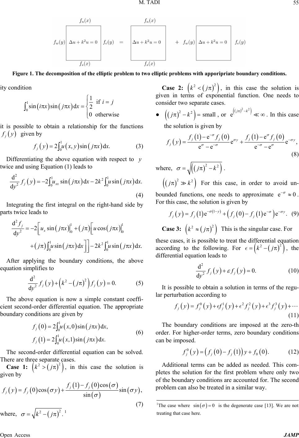

M. TADI 55

Figure 1. The decomposition of the elliptic problem to two elliptic problems with apporipriate boundary conditions.

ity condition

 

1if

sinsind 2

0otherwise

ixjx x















it is possible to obtain a relationship for the functions



y given by

 

2,sin d

yuxyjx

x (3)

Differentiating the above equation with respect to

twice and using Equation (1) leads to

  

211

200

d2sin d2sin d

djxx .

yujxxkujx

y 



(4)

Integrating the first integral on the right-hand side by

parts twice leads to

 



d2sin cos

sind2sind .

fujxjujx

ju jxxku jxx



 









 







After applying the boundary conditions, the above

equation simplifies to

 



d0.

fy kjfy

y 

(5)

The above equation is now a simple constant coeffi-

cient second-order differential equation. The appropriate

boundary conditions are given by

 

 

02 ,0sind,

12 ,1sind.

uxjx x





 (6)

The second-order differential equation can be solved.

There are three separate cases.

Case 1: , in this case the solution is

given by





kj



 

 

10cos

0cossin ,

sin

yf yy









(7)

where,



2.kj





Case 2:









, in this case the solution is

given in terms of exponential function. One needs to

consider two separate cases.

●







22smalljk , or . In this case

the solution is given by



ejk 















1e01e 0

eee e

jj jj

ff ff



 









(8)

where,

















jk For this case, in order to avoid un-

bounded functions, one needs to approximate e0







For this case, the solution is given by

 



 



1e01ee.

jj jj

fy fff



 

 (9)

Case 3:









 This is the singular case. For

these cases, it is possible to treat the dif

according to the following. For , the

differential equation leads to

ferential equation



kj

 

d0.

djj

fy fy





 (10)

It is possible to obtain a solution in terms of the regu-

lar perturbation according to

















012233

jj jjj

fyf yfyf yf y



 

(11)

The boundary conditions are imposed at the zero-th

order. For higher-order terms, zero boundary conditions

can be imposed.















01 0

jjj

fy ffyf . (12)

Additional terms can be added as needed. This com-

pletes the solution for the first problem where only two

of the boundary conditions are accounted for. The second

problem can also be treated in a similar way.

1The case where





sin 0





is the degenerate case [13]. We are not

treating that case here.

Open Access JAMP

M. TADI

3. Numerical Experiments

In this section, we use a numerical example to investigate

the applicability of the proposed method. The proposed

method is particularly useful for very high values of the

wave number. For these values none of the existing nu-

merical methods can be applied within the available

computer capacity. It is possible to use a problem for

which analytical solutions exist [2]. An exact solution for

the problem is given by

 



,coscos sinuxy kxy



 (13)

where,



is the angle of the incoming wave. Using the

exact solution one can provide the boundary conditions

for the numerical method. The domain is divided into

equal intervals in both

and . Figure 2 presents the

numerical results for . The figure shows the

error as a function of the number of orthogonal functions.

There is little dependency to the mesh size ne. The error

is the L2 norm of the difference between the numerical

result and the exact solution divide by the number of

nodes.

2000k

Figures 3-5 show the same error reduction for higher

wave numbers. Figure 3 presents the reduction in the

error for . The number of intervals is equal to

. For higher wave numbers, the same reduction

in error is observed. For higher values of k, the method

15000

k

1600

n

Figure 2. Reduction in the error as a function of the num-

ber of orthogonal functions. Other parameters are

, 2000k4



, , and the three maximum

number of orthogonal functions are .

e800n

600,800,1600

orth

n

Figure 3. Reduction in the error as a function of the num-

ber of orthogonal functions. Other parameters are

, 15000k4



, , and the three maximum

number of orthogonal functions are

e1600n

3600,

orth

n4200,4800

Figure 4． Reduction in the error as a function of the

number of orthogonal functions. Other parameters are

25000k



, 4







, e1600n



, and the three maximum

number of orthogonal functions are

6400,

orth

n7200,8400,10800





Figure 5． Reduction in the error as a function of the

number of orthogonal functions. Other parameters are

100000k



, 4







, , and the three maximum

number of orthogonal functions are

e1600n

3620022200,

orth

n30000,8400,





simply requires the inclusion of more orthogonal func-

tions in the expansion given in Equation (2). Figure 5

presents the result for and a similar reduction in

the error is obtained.

10k

The present method is particularly useful for the

Helmholtz equation at higher frequency for which exist-

ing methods require a large amount of memory. The ac-

tual calculation for the present method is done analyti-

cally in one-dimension.

4. Conclusion

In this note, we presented a numerical method for the

solution of 2-D Helmholtz equation. The method can be

applied to 3-D domains. It is based on orthogonal func-

tions. Apart from the projection of the problem onto the

space of orthogonal functions, the solution is obtained

analytically. Numerical results for a number of cases

with very high wave numbers were presented.

REFERENCES

[1] G. E. Owen, “Introduction to Electromagnetic Theory,”

Dover, New York, 2003.

[2] I. Singer and E. Turkel, “High-Order Finite Difference

Methods for the Helmholtz Equation,” Computer Meth-

Open Access JAMP

M. TADI

Open Access JAMP

ods in Applied Mechanics and Engineering, Vol. 163, No.

1-4, 1998, pp. 343-358.

http://dx.doi.org/10.1016/S0045-7825(98)00023-1

[3] M. Navabi, M. H. K. Siddiqui and J. Dargahi, “A New

9-Point Sixth-Order Accurate Compact Finite-Difference

Method for the Helmholtz Equation,” Journal of Sound

and Vibration, Vol. 307, No. 3-5, 2007, pp. 972-982.

http://dx.doi.org/10.1016/j.jsv.2007.06.070

[4] P. Nadukandi, E. Onate and J. Garcia, “A Fouth-Order

Compact Scheme for the Helmholtz Equation: Alpha-In-

terpolation and FEM and FDM Stencils,” International

Journal for Numerical Methods in Engineering, Vol. 86,

No. 1, 2011, pp. 18-46.

http://dx.doi.org/10.1002/nme.3043

[5] H. Dogan, V. Popov and E. Hin Ooi, “The Radial Basis

Integral Equation Method for Solving the Helmholtz

Equation,” Engineering Analysis with Boundary Elements,

Vol. 36, No. 6, 2012, pp. 934-943.

http://dx.doi.org/10.1016/j.enganabound.2011.12.003

[6] X. Feng and H. Wu, “hp-Discontinuous Galerkin Meth-

ods for the Helmholtz Equation with Large Wave Num-

ber,” Mathematics of Computation, Vol. 80, No. 276,

2011, pp. 1997-2024.

http://dx.doi.org/10.1090/S0025-5718-2011-02475-0

[7] G. F. Dargush and M. M. Grigoiev, “A Multi-Level

Multi-Integral Algorithm for the Helmholtz Equation,”

Proceedings of IMECE-2005, 5-11 November 2005, Or-

lando, pp. 1-8.

[8] K. Otto and E. Larsson, “Iterative Solution of the Helm-

holtz Equation by a Second-Order Method,” SIAM Jour-

nal on Matrix Analysis and Applications, Vol. 21, No. 1,

1999, pp. 209-229.

http://dx.doi.org/10.1137/S0895479897316588

[9] D. Gordon and R. Gordon, “Robust and Highly Scalable

Parallel Solution of the Helmholtz Equation with Large

Wave Numbers,” Journal of Computational and Applied

Mathematics, Vol. 237, No. 1, 2013, pp. 182-196.

http://dx.doi.org/10.1016/j.cam.2012.07.024

[10] Y. Zhuang and X. H. Sun, “A High-Order ADI Method

for Separable Generalized Helmholtz Equations,” Ad-

vances in Engineering Software, Vol. 31, No. 8-9, 2000,

pp. 585-591.

http://dx.doi.org/10.1016/S0965-9978(00)00026-0

[11] B. N. Li, L. Cheng, A. J. Deek and M. Zhao, “A Semi-

Analytical Solution Method for Two-Dimensional Helm-

holtz Equation,” Applied Oscean Research, Vol. 28, No.

3, 2006, pp. 193-207.

http://dx.doi.org/10.1016/j.apor.2006.06.003

[12] G. Bao, G. W. Wei and S. Zhao, “Numerical Solution of

the Helmholtz Equation with High Wavenumbers,” In-

ternational Journal for Numerical Methods in Engineer-

ing, Vol. 59, No. 3, 2004, pp. 389-408.

http://dx.doi.org/10.1002/nme.883

[13] Z. C. Li, “The Trefftz Method for the Helmholtz Equation

with Degeneracy,” Applied Numerical Mathematics, Vol.

58, No. 2, 2008, pp. 131-159.

http://dx.doi.org/10.1016/j.apnum.2006.11.004

Appendix

In 3-D one can assume a form given by

 

,,sin sin,

uxyzf yixjz













(14)

here, after using the orthogonality conditions, the func-

tions are given by

)( yfij

   

4,,sinsind

ij .

yuxyzixjzx

 z

(15)

Also, for the 3-D Helmholtz equation, one needs to split

the problem into three similar problems.