Elucidating General Equilibrium Multiplier Effects: A Differential Perspective

doi:10.4236/tel.2013.35046

Paper Menu >>

Journal Menu >>

Theoretical Economics Letters, 2013, 3, 279-282

http://dx.doi.org/10.4236/tel.2013.35046 Published Online October 2013 (http://www.scirp.org/journal/tel)

Elucidating General Equilibrium Multiplier Effects:

A Differential Perspective

M. Alejandro Cardenete1, Ferran Sancho2

1Department of Economics, Universidad Loyola Andalucía, Sevilla, Spain

2Department of Economics, Universitat Autònoma de Barcelona, Barcelona, Spain

Email: [email protected], [email protected]

Received August 20, 2013; revised September 11, 2013; accepted September 18, 2013

Attribution License, which permits unrestricted use, distribution, and reproduction in any medium, provided the original work is

properly cited.

ABSTRACT

Expenditure multipliers are routinely used to evaluate the effectiveness of government spending. When interested in

disaggregated effects, interindustry models provide the necessary tools to be able to look at very detailed sectorial re-

sults. These models are theoretically simple and empirically operational, which makes them easily implementable and

therefore popular with policy makers. They miss, however, quite a bit of the interaction that takes place at the micro

level. On the one hand, they ignore the role exerted by supply constraints in primary factors; on the other hand, they

look at the world as though it is fully linear. We overcome these limitations by using an opposite Walrasian general

equilibrium model to compute marginal multipliers. By using differential calculus, we also offer some insights regard-

ing the “under-the-hood” circuits of influence.

Keywords: Marginal Multipliers; General Equilibrium; Linear vs. Nonlinear Models

1. Introduction

Let us begin by considering the general setup of an eco-

nomy described by m endogenous variables and k exter-

nal exogenous variables, (say, policy instruments) affect-

ing the equilibrium state. In this economy, multipliers

connect exogenous injections xi (I = 1,2 ··· k) with en-

dogenous responses ej (j = 1,2 ··· m). If the vector func-

tion :mk m



(, )ex R represents the equilibrium state

, then it is possible to use differential calcu-

lus [1] to study the equilibrium dependence of endoge-

nous variables e with respect to exogenous one x. In this

case, we would have

eF







,,deFex edeFex Xdx  .

Solving now for de would yield



(, )

deFexe Fexxdx

exdx







where M is a (m × k) matrix whose generic element

∂ej/∂xi = mji(e, x) is an estimate of the (marginal) multi-

plier effect exerted by injection xi upon endogenous

variable ej. Notice that in principle the multiplier matrix,

M itself may be variable since it depends on the particu-

lar equilibrium state e induced by instruments x and the

characteristics of the economy, as embodied in F. Since

the vector function F is not usually directly observable,

neither are its derivatives nor is matrix M, hence there is

the need for relying on some type of approximation. One

such approximation is to linearize the economy; another

is to use numerical methods for the evaluation of nonlin-

ear equilibrium relationships.

2. Linear Multipliers

We now consider a linear economy of the interindustry

type. For this type of economies we have n endogenous

(m = n) and n exogenous variables (k = n). The endoge-

nous variables correspond to total output in each of the n

sectors, whereas the exogenous variables describe final

demand. This includes discretional government demand

for the goods and services of each of the n sectors. We

will use the n-vector q to denote output (i.e. e = q now)

and keep x for the exogenous variables. The equilibrium

state for this linear economy is represented, again using

the vector function F, by q = F(q, x). Thanks to the line-

arity assumption this can be seen to adopt the form q =

Aq + x, where A is a n×n nonnegative, productive and

homothetic technical coefficient matrix. From the equi-

M. A. CARDENETE, F. SANCHO

280

librium state we can quickly write the reduced form

linking output with instruments as q = (I − A)−1x = Mx,

with M representing the multiplier matrix of the linear

economy. Because of the assumptions on A, the matrix

M is constant. Its entries are independent of the equilib-

rium state. Taking derivatives, it is quite simple now to

relate changes in output with external changes in instru-

ments





  IA Mx



(1)

Multipliers are given directly by the cells in matrix M,

i.e. ∂qj/∂xi = mji. All that is needed to compute (linear)

multipliers is the coefficients matrix A. Since this matrix

is readily available from official statistics, this explains

the popularity of linear models in policy oriented em-

pirical economics. Even more, linear models are so sim-

ple that we need not worry about prices. Prices, in fact,

can be seen to be completely independent from quantities

in linear interindustry models. Notice that if quantities

are not affected by prices, neither are multipliers. End of

the story, all needed multiplier information is contained

in matrix M. But we know that the actual story is bit

more complicated than that since, in general, prices and

quantities are mutually dependent.

3. Applied General Equilibrium Mul tip li ers

In a standard general equilibrium model the interactions

of supply and demand determine, at the same time, prices

and quantities. We use now a general equilibrium frame-

work to elucidate multipliers and compare them to their

linear counterpart. Endogenous variables include now n

output levels q and n prices p, that is, , so in

total we have 2n endogenous variables. Let us consider

again that the government decides how much to buy of

each of the n goods and services; the government’s de-

mand levels are denoted by the vector x representing

policy instruments. The structural function F represent-

ing the equilibrium state would now be of the type



,eqp

:nn n



which in turn can be split in two func-

tions n n

R and 2

nn n



R determin-

ing quantities and prices, respectively. The complete

general equilibrium state is represented by (q, p) = F(q, p,

x), or using the fact that

FF, it can also be seen



pFqpx

qFqpx



 (2)

We perform comparative statics on the equilibrium

state represented in Equation (2) considering an exoge-

nous change dx in the instruments x. We would obtain

qq qp qx

pq pp px

dqMdq Mdp Mdx

dpM dqM dpMdx



 (3)

where we use, in Equation (3), the notational convention





Fqpxq



,



Fqpxp , and so

on. Solving for dp in the second expression in Equation

(3) and substituting the result in the first equation would

yield





qq qp qx

qqqp pppq px

qq qppppq

qx qppppx

dqMdq Mdp Mdx



dq MIMMdq Mdx

Mdx

MMIM Mdq

MMIM Mdx







 







 









 





(4)

Solving now for dq in Equation (4) we finally obtain













1,,

qq qppppq

qx qppppx

dqIMMI MM

MIM Mqpxdx



 





 





(5)

where





,,qpxM

stands for the general quantity mul-

tiplier matrix1. We now proceed to relate the linear mul-

tiplier matrix in Equation (1) with the general multi-

plier matrix





,,xqpM derived in Equation (5).

Recall first that in linear models quantities and prices

are independently determined. Under this assumption the

partial derivative matrices Mpq and Mqp would be such

that Mpq = Mqp = 0 and then Equation (5) can be easily

verified to reduce to





qq qx

dqIMM dx



 (6)

The simplified expression that appears in Equation (6)

is of course the differential version of the classical linear

multiplier expression picked up in Equation (1) above,

with Mqq = A and Mqxdx = Δx. The chains of interactions,

however, can be seen to be quite more complex in Equa-

tion (5) than in Equation (1), in accordance with the

higher complexity of nonlinear models vis-a-vis linear

ones.

Figure 1 below depicts the way the model’s intercon-

nections work. Facing an external disturbance in x, the

system first reacts with changes in prices and quantities

through matrices Mpx and Mqx. Price effects repeatedly

self multiply through the loop Mpp along the cost struc-

ture which, in turn, are affected by cross effects Mqp from

quantities to prices. Similarly, the initial effect of the

disturbance on quantities gets itself multiplied by the

chain reaction that moves directly from quantities to

quantities, i.e. Mqq, and indirectly from quantities to

looped prices and back to quantities via the combined

1A similar derivation, that we omit, would produce a general price

multiplier matrix.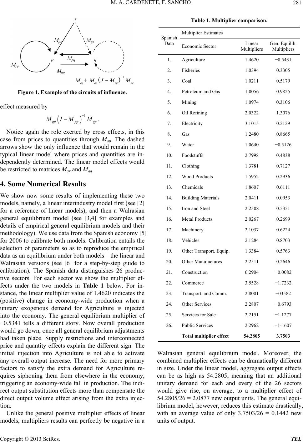

M. A. CARDENETE, F. SANCHO 281

Figure 1. Example of the circuits of influence.

effect measured by



qppp qp

IM M



.

Notice again the role exerted by cross effects, in this

case from prices to quantities through Mqp. The dashed

arrows show the only influence that would remain in the

typical linear model where prices and quantities are in-

dependently determined. The linear model effects would

be restricted to matrices Mqx and Mqq.

4. Some Numerical Results

We show now some results of implementing these two

models, namely, a linear interindustry model first (see [2]

for a reference of linear models), and then a Walrasian

general equilibrium model (see [3,4] for examples and

details of empirical general equilibrium models and their

methodology). We use data from the Spanish economy [5]

for 2006 to calibrate both models. Calibration entails the

selection of parameters so as to reproduce the empirical

data as an equilibrium under both models—the linear and

Walrasian versions (see [6] for a step-by-step guide to

calibration). The Spanish data distinguishes 26 produc-

tive sectors. For each sector we show the multiplier ef-

fects under the two models in Table 1 below. For in-

stance, the linear multiplier value of 1.4620 indicates the

(positive) change in economy-wide production when a

unitary exogenous demand for Agriculture is injected

into the economy. The general equilibrium multiplier of

−0.5341 tells a different story. Now overall production

would go down, once all general equilibrium adjustments

had taken place. Supply restrictions and interconnected

price and quantity effects explain the different sign. The

initial injection into Agriculture is not able to activate

any overall output increase. The need for more primary

factors to satisfy the extra demand for Agriculture re-

quires siphoning them from elsewhere in the economy,

triggering an economy-wide fall in production. The indi-

rect output substitution effects more than compensate the

direct output volume effect arising from the extra injec-

tion.

Unlike the general positive multiplier effects of linear

models, multipliers results can perfectly be negative in a

Table 1. Multiplier comparison.

Multiplier Estimates

Spanish

Data Economic Sector Linear

Multipliers

Gen. Equilib.

Multipliers

1. Agriculture 1.4620 −0.5431

2. Fisheries 1.0394 0.3305

3. Coal 1.0211 0.5179

4. Petroleum and Gas 1.0056 0.9825

5. Mining 1.0974 0.3106

6. Oil Refining 2.0322 1.3076

7. Electricity 3.1015 0.2129

8. Gas 1.2480 0.8665

9. Water 1.0640 −0.5126

10. Foodstuffs 2.7998 0.4838

11. Clothing 1.3781 0.7127

12. Wood Products 1.5952 0.2936

13. Chemicals 1.8607 0.6111

14. Building Materials 2.0411 0.0953

15. Iron and Steel 2.2508 0.5351

16. Metal Products 2.0267 0.2699

17. Machinery 2.1037 0.6224

18. Vehicles 2.1284 0.8703

19. Other Transport. Equip. 1.3384 0.5763

20. Other Manufactures 2.2511 0.2646

21. Construction 6.2904 −0.0082

22. Commerce 3.5528 −1.7232

23. Transport. and Comm. 2.8001 −03582

24. Other Services 2.2807 −0.6793

25. Services for Sale 2.2151 −1.1277

26. Public Services 2.2962 −1-1607

Total multiplier effect 54.2805 3.7503

Walrasian general equilibrium model. Moreover, the

combined multiplier effects can be dramatically different

in size. Under the linear model, aggregate output effects

can be as high as 54.2805, meaning that an additional

unitary demand for each and every of the 26 sectors

would give rise, on average, to a multiplier effect of

54.2805/26 = 2.0877 new output units. The general equi-

librium model, however, reduces this estimate drastically,

with an average value of only 3.7503/26 = 0.1442 new

units of output.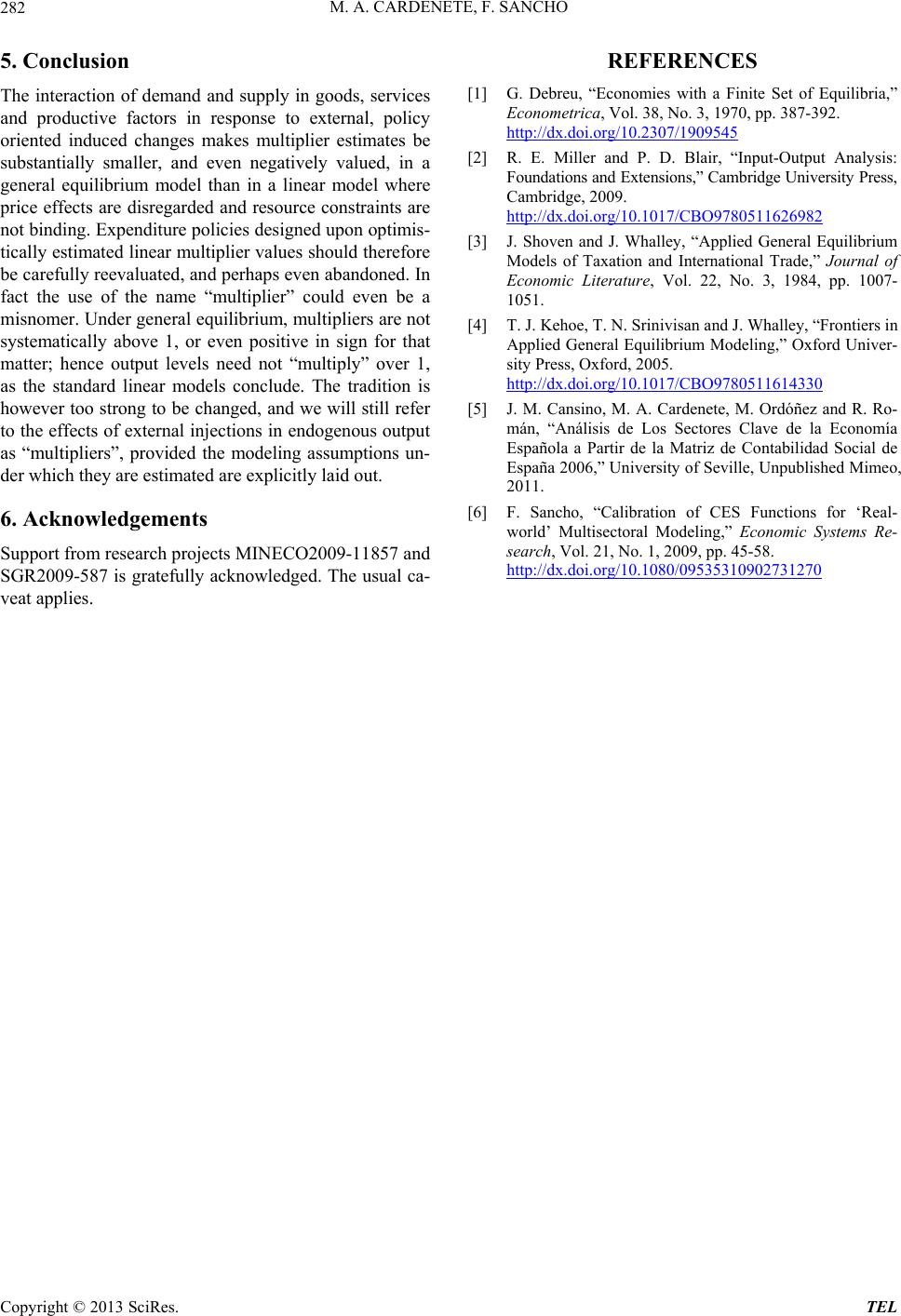

M. A. CARDENETE, F. SANCHO

282

5. Conclusion

The interaction of demand and supply in goods, services

and productive factors in response to external, policy

oriented induced changes makes multiplier estimates be

substantially smaller, and even negatively valued, in a

general equilibrium model than in a linear model where

price effects are disregarded and resource constraints are

not binding. Expenditure policies designed upon optimis-

tically estimated linear multiplier values should therefore

be carefully reevaluated, and perhaps even abandoned. In

fact the use of the name “multiplier” could even be a

misnomer. Under general equilibrium, multipliers are not

systematically above 1, or even positive in sign for that

matter; hence output levels need not “multiply” over 1,

as the standard linear models conclude. The tradition is

however too strong to be changed, and we will still refer

to the effects of external injections in endogenous output

as “multipliers”, provided the modeling assumptions un-

der which they are estimated are explicitly laid out.

6. Acknowledgements

Support from research projects MINECO2009-11857 and

SGR2009-587 is gratefully acknowledged. The usual ca-

veat applies.

REFERENCES

[1] G. Debreu, “Economies with a Finite Set of Equilibria,”

Econometrica, Vol. 38, No. 3, 1970, pp. 387-392.

http://dx.doi.org/10.2307/1909545

[2] R. E. Miller and P. D. Blair, “Input-Output Analysis:

Foundations and Extensions,” Cambridge University Press,

Cambridge, 2009.

http://dx.doi.org/10.1017/CBO9780511626982

[3] J. Shoven and J. Whalley, “Applied General Equilibrium

Models of Taxation and International Trade,” Journal of

Economic Literature, Vol. 22, No. 3, 1984, pp. 1007-

1051.

[4] T. J. Kehoe, T. N. Srinivisan and J. Whalley, “Frontiers in

Applied General Equilibrium Modeling,” Oxford Univer-

sity Press, Oxford, 2005.

http://dx.doi.org/10.1017/CBO9780511614330

[5] J. M. Cansino, M. A. Cardenete, M. Ordóñez and R. Ro-

mán, “Análisis de Los Sectores Clave de la Economía

Española a Partir de la Matriz de Contabilidad Social de

España 2006,” University of Seville, Unpublished Mimeo,

2011.

[6] F. Sancho, “Calibration of CES Functions for ‘Real-

world’ Multisectoral Modeling,” Economic Systems Re-

search, Vol. 21, No. 1, 2009, pp. 45-58.

http://dx.doi.org/10.1080/09535310902731270