Estimation of Longitudinal Tire Force Using Nonlinearity Observer

doi:10.4236/ojapps.2013.32B008

Paper Menu >>

Journal Menu >>

Open Journal of Applied Sciences, 2013, 3, 41-46

doi:10.4236/ojapps.2013.32B008 Published Online June 2013 (http://www.scirp.org/journal/ojapps)

Estimation of Longitudinal Tire Force Using

Nonlinearity Observer

Suwat Kuntanapreeda

Department of Mechanical and Aerospace Engineering, Faculty of Engineering,

King Mongkut’s University of Technology North Bangkok, Bangkok, Thailand

Email: [email protected]

Received 2013

ABSTRACT

Tire forces are the major forces propelling the road vehicles. They significantly affect the dynamic behavior of the ve-

hicles. Estimation of the tire forces is essential in vehicle dynamics and control. This paper presents an observer-based

scheme for estimation of the longitudinal tire force of electric vehicles in real time. The observer is based on a

nonlinearity observer method. The pole-placement technique is used for determination of the observer gains. Simulation

results demonstrate that the observer is able to estimate the tire force successfully. The experiments are implemented on

a single-wheel electric vehicle test rig. The test rig comprises an electric motor driven wheel and a free-rolling drum

simulating vehicle-on-road situations. Experimental results confirm the effectiveness of the present scheme.

Keywords: Estimation; Nonlinearity Observer; Tire Force; Traction Control; Electric Vehicles

1. Introduction

Electric vehicles (EVs) have become very attractive for

replacing conventional internal combustion engine vehi-

cles because of environmental and energy problems [1].

The research and development of EVs and hybrid EVs

have been investigated on various topics such as, for

example, propulsion systems [2], power converters [3],

and motion control [4].

Traction control plays an important role in vehicle mo-

tion control because it increases drive efficiency, safety,

and stability. Tire forces are essential in traction control.

They are the vehicular propulsive forces produced by

friction between the rolling wheel and the road surface.

The characteristic of the friction between the wheel and

the road surface is very nonlinear. It mainly depends on

the wheel slip and the tire/road surface condition. In [5],

an approach to estimate the tire-road friction during

normal drive is presented. The approach is based on a

Kalman filter to give estimates of the slip-slope. In [6],

an on-line least-squares method is used to estimate the

parameters concerned with a friction force margin. The

effect of the estimation is evaluated by applying the

method to the breaking control. A slip-based method to

estimate the maximum available tire-road friction during

breaking is developed in [7]. The method is based on the

hypothesis that the slope of the slip curve at the low-slip

region during normal driving can indicate the maximum

friction coefficient. In [8], vehicle-dynamics-based

methods for tire-road friction coefficients estimation are

reviewed. The methods include slip-slope-based, lateral-

ehicle-dynamics-based, and an EKF-based estimation

methods. In [9], three different observers are developed

for the estimation of slip ratios and longitudinal tire

forces. The observers include one that utilizes engine

torque, break torque, and GPS measurements, one that

utilizes torque measurements and an accelerometer, and

one that utilizes GPS measurements and an accelerome-

ter.

This paper presents an observer-based scheme for es-

timation of the longitudinal tire force of EVs using a

nonlinearity observer. Simulation and experimental stud-

ies are used to illustrate the effectiveness of the present

scheme. A single-wheel test rig is used as an experimen-

tal test bench.

2. Nonlinearity Observer

The nonlinearity observer developed in [10,11] is re-

viewed in this section. Consider the following nonlinear

system

()()( (),)()

() ()

tt tt







xAxNfx Bu

yCx



(1)

where , , and are, respectively, the state vector,

the control vector, and the output vector, respectively.

, , and are, respectively, the system ma-

trix, the control input matrix, the output matrix, and the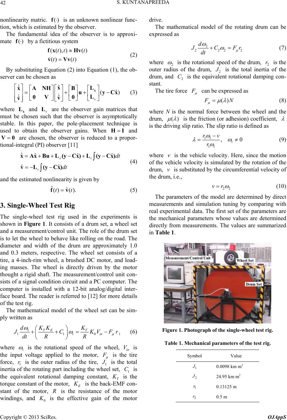

NA B

S. KUNTANAPREEDA

nonlinearity matric. is an unknown nonlinear func-

tion, which is estimated by the observer.

()f

(()

()











The fundamental idea of the observer is to approxi-

mate by a fictitious system

()f

,) ()

()

tt t

Hv

vVv (2)

By substituting Equation (2) into Equation (1), the ob-

server can be chosen as

ˆˆ

(

ˆv

 





 









xA B

uyC

0V 0



)



(3)

where x and v are the observer gain matrices that

must be chosen such that the observer is asymptotically

stable. In this paper, the pole-placement technique is

used to obtain the observer gains. When

L L



and

are chosen, the observer is reduced to a propor-

tional-integral (PI) observer [11]

V0

ˆˆˆ ˆ

 





xAxB (yCx)L(yCx)

vL x)







(yC

ˆ()f

(4)

and the estimated nonlinearity is given by

ˆ().ttv

(5)

3. Single-Wheel Test Rig

The single-wheel test rig used in the experiments is

shown in Figure 1. It consists of a drum set, a wheel set

and a measurement/control unit. The role of the drum set

is to let the wheel to behave like rolling on the road. The

diameter and width of the drum are approximately 1.0

and 0.3 meters, respective. The wheel set consists of a

tire, a 4-inch-rim wheel, a brushed DC motor, and load-

ing masses. The wheel is directly driven by the motor

thought a rigid shaft. The measurement/control unit con-

sists of a signal condition circuit and a PC computer. The

computer is installed with a 12-bit analog/digital inter-

face board. The reader is referred to [12] for more details

of the test rig.

The mathematical model of the wheel set can be sim-

ply written as

11101

dK K

CKVFr

dt RR







 





 (6)

where 1



is the rotational speed of the wheel, in

V is

the input voltage applied to the motor,



is the tire

force, 1 is the outer radius of the tire, 1

is the total

inertia of the rotating part including the wheel set, 1 is

the equivalent rotational damping constant, T

is the

torque constant of the motor,

is the back-EMF con-

stant of the motor, is the resistance of the motor

windings, and

is the effective gain of the motor

drive.

The mathematical model of the rotating drum can be

expressed as

222





r (7)

where 2



is the rotational speed of the drum, 2 is the

outer radius of the drum, 2

is the total inertia of the

drum, and is the equivalent rotational damping con-

stant.

The tire force



can be expressed as

()







(8)

where N is the normal force between the wheel and the

drum, ()





is the friction (or adhesion) coefficient,



is the driving slip ratio. The slip ratio is defined as







0





 (9)

where is the vehicle velocity. Here, since the motion

of the vehicle velocity is simulated by the rotation of the

drum, is substituted by the circumferential velocity of

the drum, i.e.,



 (10)

The parameters of the model are determined by direct

measurements and simulation tuning by comparing with

real experimental data. The first set of the parameters are

the mechanical parameters whose values are determined

directly from measurements. The values are summarized

in Table 1.

Figure 1. Photograph of the single-wheel test rig.

Table 1. Mechanical parameters of the test rig.

Symbol Value

J 0.0098 km m2

J 24.95 km m2

r0.13125 m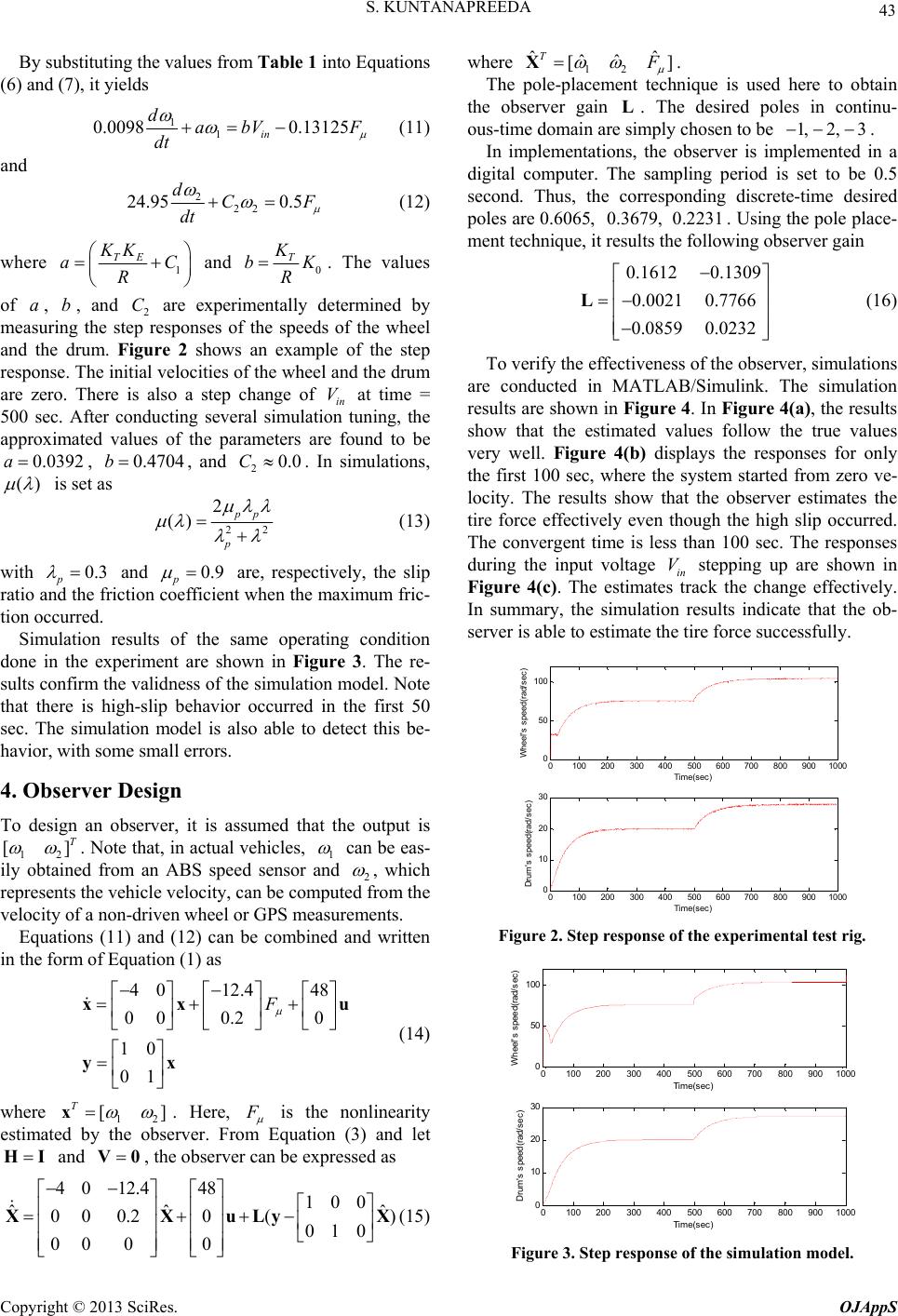

r 0.5 m

S. KUNTANAPREEDA 43

By substituting the values from Table 1 into Equations

(6) and (7), it yields

0.0098 0.13125

dabV F





  (11)

and

24.95 0.5

dt F





 (12)

where 1









and 0

K

. The values

of , , and 2 are experimentally determined by

measuring the step responses of the speeds of the wheel

and the drum. Figure 2 shows an example of the step

response. The initial velocities of the wheel and the drum

are zero. There is also a step change of in at time =

500 sec. After conducting several simulation tuning, the

approximated values of the parameters are found to be

, , and . In simulations,

0.

()

0392

0.47

a04b20.0C





is set as

() pp





(13)







with 0.3



 and 0.9



 are, respectively, the slip

ratio and the friction coefficient when the maximum fric-

tion occurred.

Simulation results of the same operating condition

done in the experiment are shown in Figure 3. The re-

sults confirm the validness of the simulation model. Note

that there is high-slip behavior occurred in the first 50

sec. The simulation model is also able to detect this be-

havior, with some small errors.

4. Observer Design

To design an observer, it is assumed that the output is

]



. Note that, in actual vehicles, 1



can be eas-

ily obtained from an ABS speed sensor and 2



, which

represents the vehicle velocity, can be computed from the

velocity of a non-driven wheel or GPS measurements.

Equations (11) and (12) can be combined and written

in the form of Equation (1) as

40 12.448

00 0.20







 











u

]

(14)

where 12

[



x. Here,



is the nonlinearity

estimated by the observer. From Equation (3) and let

and , the observer can be expressed as

HI V0

4 012.448100

ˆˆˆ

00 0.20()

010

00 00





















XXuL

(15)

where 12

ˆˆ

[]





X.

The pole-placement technique is used here to obtain

the observer gain L. The desired poles in continu-

ous-time domain are simply chosen to be .

1, 2, 3 

In implementations, the observer is implemented in a

digital computer. The sampling period is set to be 0.5

second. Thus, the corresponding discrete-time desired

poles are 0.60 . Using the pole place-

ment technique, it results the following observer gain

65,0.3679, 0.2231

0.1612 0.1309

0.0021 0.7766

0.0859 0.0232



























L (16)

To verify the effectiveness of the observer, simulations

are conducted in MATLAB/Simulink. The simulation

results are shown in Figure 4. In Figure 4(a), the results

show that the estimated values follow the true values

very well. Figure 4(b) displays the responses for only

the first 100 sec, where the system started from zero ve-

locity. The results show that the observer estimates the

tire force effectively even though the high slip occurred.

The convergent time is less than 100 sec. The responses

during the input voltage in stepping up are shown in

Figure 4(c). The estimates track the change effectively.

In summary, the simulation results indicate that the ob-

server is able to estimate the tire force successfully.

0100 200 300 400 500 600 700 800900 1000

100

Ti me( sec)

Wheel's speed(rad/sec)

0100 200 300 400 500 600 700 800900 1000

Ti me( sec)

Drum's speed(rad/sec)

Figure 2. Step response of the experimental test rig.

0100 200300 400 500600 700 800900 1000

100

Time(sec)

Wheel's speed(rad/sec)

0100 200300 400 500600 700 800900 1000

Time(sec)

Drum's speed(rad/sec)

Figure 3. Step response of the simulation model.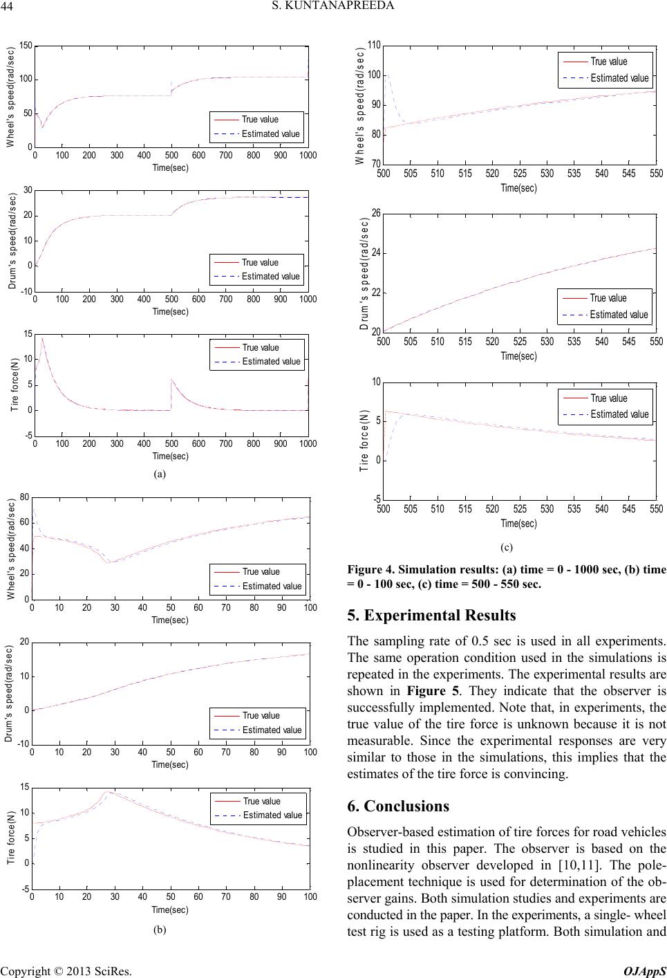

S. KUNTANAPREEDA

0100 200300 400500 600 700800 9001000

100

150

Time(sec)

Wheel's speed(rad/sec)

True value

Estimated value

0100 200300 400500 600 700800 9001000

-10

Time(sec)

Drum's speed(rad/sec)

True value

Estimated value

0100 200300 400500 600 700800 9001000

-5

Time(sec)

Tire force(N)

True value

Estimated value

(a)

010 2030 4050 60 70 80 90 100

Time(sec)

Wheel's speed(rad/sec)

True value

Estimated value

010 2030 4050 60 70 80 90 100

-10

Time(sec)

Drum's speed(rad/sec)

True value

Estimated value

010 2030 4050 60 70 80 90 100

-5

Time(sec)

Tire force(N)

True value

Estimated value

(b)

500 505 510515 520 525 530 535540 545550

100

110

Time(sec)

Wheel's speed(rad/sec)

True value

Estimated value

500 505 510515 520 525 530 535540 545550

Time(sec)

Drum's speed(rad/sec)

True value

Estimated value

500 505 510515 520 525 530 535540 545550

-5

Time(sec)

Tire force(N)

True value

Estimated value

(c)

Figure 4. Simulation results: (a) time = 0 - 1000 sec, (b) time

= 0 - 100 sec, (c) time = 500 - 550 sec.

5. Experimental Results

The sampling rate of 0.5 sec is used in all experiments.

The same operation condition used in the simulations is

repeated in the experiments. The experimental results are

shown in Figure 5. They indicate that the observer is

successfully implemented. Note that, in experiments, the

true value of the tire force is unknown because it is not

measurable. Since the experimental responses are very

similar to those in the simulations, this implies that the

estimates of the tire force is convincing.

6. Conclusions

Observer-based estimation of tire forces for road vehicles

is studied in this paper. The observer is based on the

nonlinearity observer developed in [10,11]. The pole-

placement technique is used for determination of the ob-

server gains. Both simulation studies and experiments are

conducted in the paper. In the experiments, a single- wheel

test rig is used as a testing platform. Both simulation and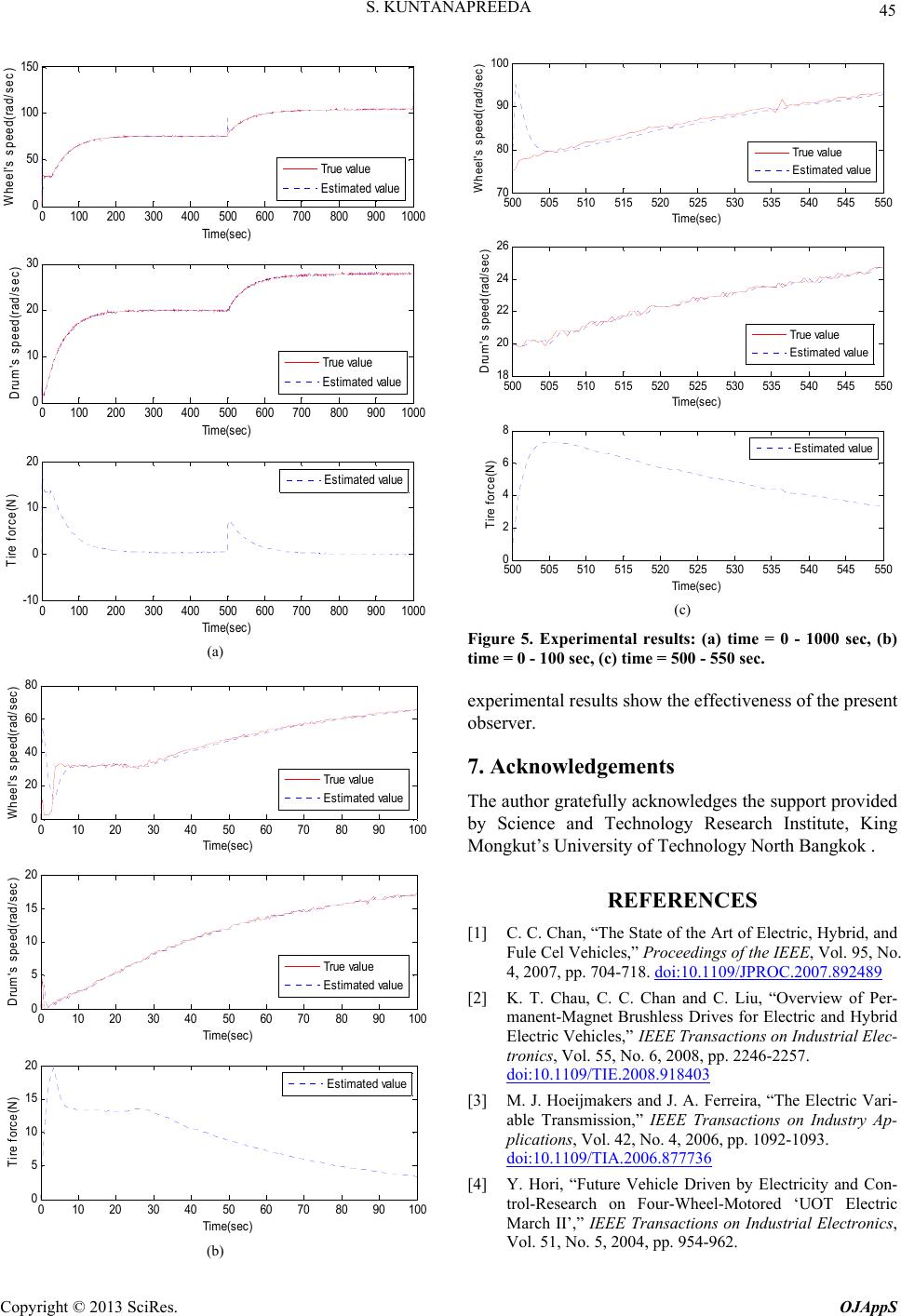

S. KUNTANAPREEDA 45

0100 200300 400500 600 700800 900 1000

100

150

Ti me(s ec )

Wheel's speed(rad/sec)

True value

Estimated value

0100 200300 400500 600 700800 900 1000

Ti me(s ec )

Drum's speed(rad/sec)

True value

Estimated value

0100 200300 400500 600 700800 900 1000

-10

Ti me(s ec )

Tire force(N)

Estimated value

(a)

0102030405060 708090 100

Time ( sec)

Wheel's speed(rad/sec)

True value

Estimated value

0102030405060 708090 100

Time ( sec)

Drum's speed(rad/sec)

True value

Estimated value

0102030405060 708090 100

Time ( sec)

Tire force(N)

Estimated value

(b)

500 505 510 515 520525 530 535540 545 550

100

Time (sec)

Wheel's speed(rad/sec)

True value

Estimated value

500 505 510 515 520525 530 535540 545 550

Time (sec)

Drum's speed(rad/sec)

True value

Estimated value

500 505 510 515 520525 530 535540 545 550

Time (sec)

Tire force(N)

Estimated value

(c)

Figure 5. Experimental results: (a) time = 0 - 1000 sec, (b)

time = 0 - 100 sec, (c) time = 500 - 550 sec.

experimental results show the effectiveness of the present

observer.

7. Acknowledgements

The author gratefully acknowledges the support provided

by Science and Technology Research Institute, King

Mongkut’s University of Technology North Bangkok .

REFERENCES

[1] C. C. Chan, “The State of the Art of Electric, Hybrid, and

Fule Cel Vehicles,” Proceedings of the IEEE, Vol. 95, No.

4, 2007, pp. 704-718. doi:10.1109/JPROC.2007.892489

[2] K. T. Chau, C. C. Chan and C. Liu, “Overview of Per-

manent-Magnet Brushless Drives for Electric and Hybrid

Electric Vehicles,” IEEE Transactions on Industrial Elec-

tronics, Vol. 55, No. 6, 2008, pp. 2246-2257.

doi:10.1109/TIE.2008.918403

[3] M. J. Hoeijmakers and J. A. Ferreira, “The Electric Vari-

able Transmission,” IEEE Transactions on Industry Ap-

plications, Vol. 42, No. 4, 2006, pp. 1092-1093.

doi:10.1109/TIA.2006.877736

[4] Y. Hori, “Future Vehicle Driven by Electricity and Con-

trol-Research on Four-Wheel-Motored ‘UOT Electric

March II’,” IEEE Transactions on Industrial Electronics,

Vol. 51, No. 5, 2004, pp. 954-962.

S. KUNTANAPREEDA

doi:10.1109/TIE.2004.834944

[5] F. Gustafsson, “Slip-Based Tire-Road Friction Estima-

tion,” Automatica, Vol. 33, No. 6, 1997, pp. 1087-1099.

doi:10.1016/S0005-1098(97)00003-4

[6] E. Ono, K. Asano, M. Sugai, S. Ito, M. Yamamoto, M.

Sawada and Y. Yasui, “Estimation of Automotive Tire

Force Chraracteristics Using Wheel Velocity,” Control

Engineering Practice, Vol. 11, 2003, pp. 1361-1370.

doi:10.1016/S0967-0661(03)00073-X

[7] S. Müller, M. Uchanski and K. Hedrick, “Estimation of

the Maximum Tire-Road Friction Coefficient,” ASME J.

Dynamic Systems, Measurement, and Control, Vol. 125,

2003, pp. 607-617. doi:10.1115/1.1636773

[8] R. Rajamani, D. Piyabongkarn, J. Y. Lew, K. Yi and G.

Phanomchoeng, “Tire-Road Friction-Coefficient Estima-

tion,” IEEE Control Systems Magazine, Vol. 30, No. 4,

2010, pp. 54-69. doi:10.1109/MCS.2010.937006

[9] R. Rajamani, G. Phanomchoeng, D. Piyabongkarn and J.

Y. Lew, “Algorithms for Real-Time Estimation of Indi-

vidual Wheel Tire-Road Friction Coefficients,”

IEEE/ASME Trans. Mechatronics, Vol. 17, No. 6, 2012,

pp.1183-1195.

[10] P. C. Müller, “Estimation and Compensation of Nonlin-

earities,” Proceedings of the 1st Asian Control Confer-

ence, Tokyo, 1994, Vol. II, pp. 641-644.

[11] D. Söffker, T. J. Yu and P. C. Müller, “State Estimation

of Dynamical Systems with Nonlinearities by Using Pro-

Portional-Integral Observer,” International Journal of

Systems Science, Vol. 26, 1995, pp. 1571-1582.

doi:10.1109/MCS.2010.937006

[12] A. Kraithaisri, S. Kuntanapreeda and S. Koetniyom, “De-

velopment of A Single-Wheel Test Rig for Traction Dy-

namics and Control of Electric Vehicles,” Proceedings of

the 2012 Hong Kong International Conference on Engi-

neering and Applied Science, 2012, pp. 360-367.