Similarity Study on Snowdrift Wind Tunnel Test

doi:10.4236/ojce.2013.33B003

Paper Menu >>

Journal Menu >>

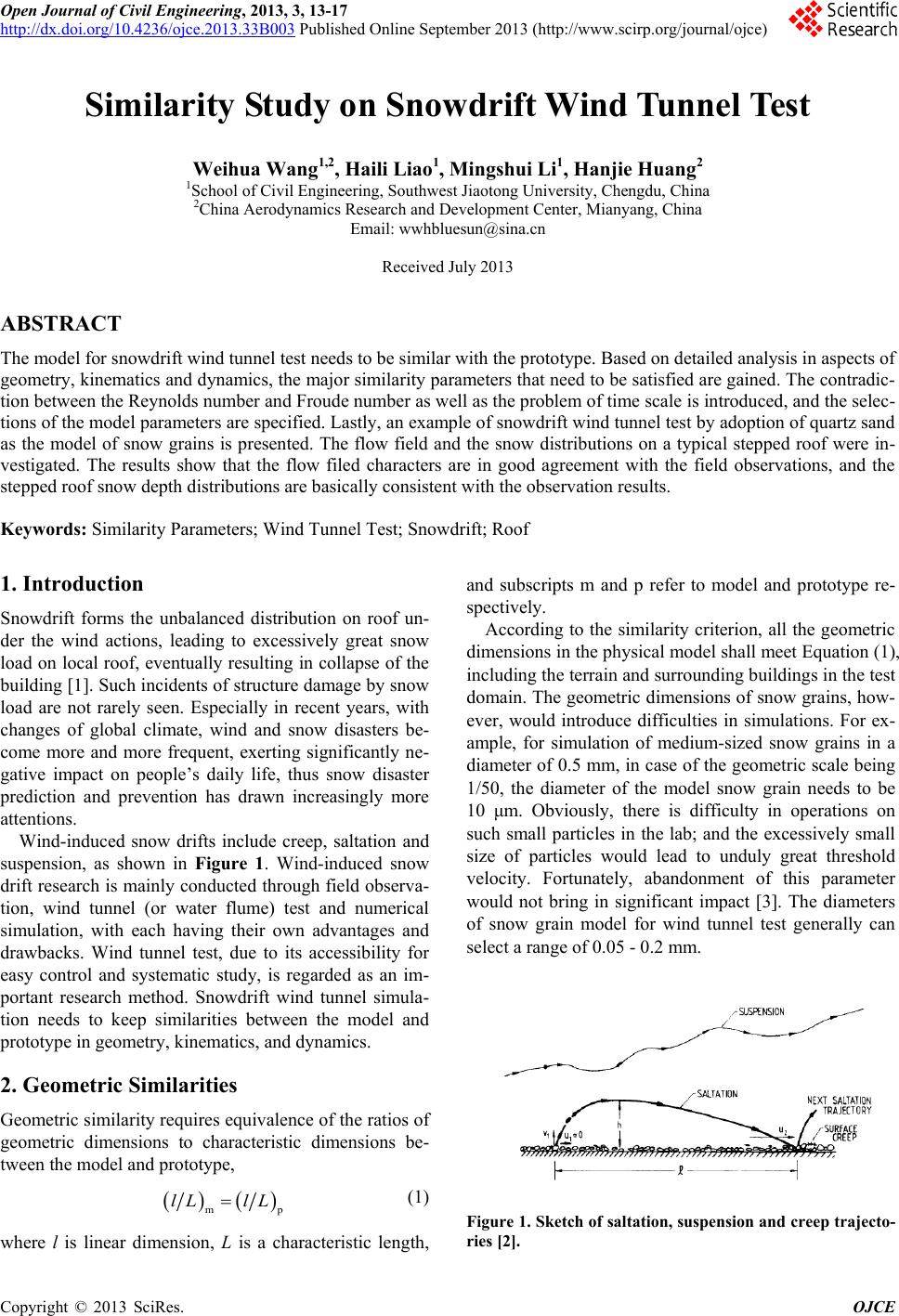Open Journal of Civil Engineering, 2013, 3, 13-17

http://dx.doi.org/10.4236/ojce.2013.33B003 Published Online September 2013 (http://www.scirp.org/journal/ojce)

Similarity Study on Snowdri ft Win d Tunnel Test

Weihua Wang1,2, Haili Liao1, Mingshui Li1, Hanjie Huang2

1School of Civil Engineering, Southwest Jiaotong University, Chengdu, China

2China Aerodynamics Research and Development Center, Mianyang, China

Email: [email protected]

Received July 2013

ABSTRACT

The model for snowdrift wind tunnel test needs to be similar with the prototype. Based on detailed analysis in aspects of

geometry, kinematics and dynamics, the major similarity parameters that need to be satisfied are gained. The contradic-

tion between the Reynolds number and Froude number as well as the problem of time scale is introduced, and the selec-

tions of the model parameters are specified. Lastly, an example of snowdrift wind tunnel test by adoption of quartz sand

as the model of snow grains is presented. The flow field and the snow distributions on a typical stepped roof were in-

vestigated. The results show that the flow filed characters are in good agreement with the field observations, and the

stepped roof snow depth distributions are basically consistent with the observation results.

Keywords: Simi larity Parameters; Wind Tunnel Test; Snowdrift; Roof

1. Introduction

Snowdrift forms the unbalanced distribution on roof un-

der the wind actions, leading to excessively great snow

load on local roof, eventually resulting in collapse of the

building [1]. Such incidents of structure damage by snow

load are not rarely seen. Especially in recent years, with

changes of global climate, wind and snow disasters be-

come more and more frequent, exerting significantly ne-

gative impact on people’s daily life, thus snow disaster

prediction and prevention has drawn increasingly more

attentions.

Wind-induced snow drifts include creep, saltation and

suspension, as shown in Figure 1. Wind-induced snow

drift research is mainly conducted through field observa-

tion, wind tunnel (or water flume) test and numerical

simulation, with each having their own advantages and

drawbacks. Wind tunnel test, due to its accessibility for

easy control and systematic study, is regarded as an im-

portant research method. Snowdrift wind tunnel simula-

tion needs to keep similarities between the model and

prototype in geometry, kinematics, and dynamics.

2. Geometric Similarities

Geometric similarity requir es equivalence of the ratios of

geometric dimensions to characteristic dimensions be-

tween the model and prototype,

( )( )

lL lL=

(1)

where l is linear dimension, L is a characteristic length,

and subscripts m and p refer to model and prototype re-

spectively.

According to the similarity criterion, all the geometric

dimensions in the physical model shall meet Equation (1),

including the terrain and surrounding buildings in the test

domain. The geometric dimensions of snow grains, how-

ever, would introduce difficulties in simulations. For ex-

ample, for simulation of medium-sized snow grains in a

diameter of 0.5 mm, in case of the geometric scale being

1/50, the diameter of the model snow grain needs to be

10 μm. Obviously, there is difficulty in operations on

such small particles in the lab; and the excessively small

size of particles would lead to unduly great threshold

velocity. Fortunately, abandonment of this parameter

would not bring in significant impact [3]. The diameters

of snow grain model for wind tunnel test generally can

select a range of 0.05 - 0.2 mm.

Figure 1. Sketch of saltation, suspension and creep trajecto-

ries [2].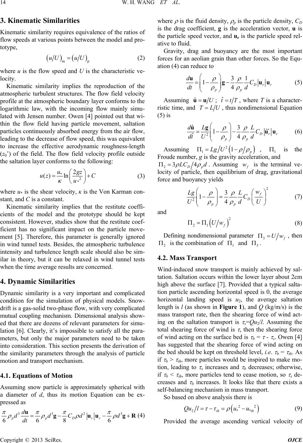

W. H. WANG ET AL.

3. Kinematic Similarities

Kinematic similarity requires equivalence of the ratio s of

flow speeds at various points between the model and pro-

totype,

( )( )

uU uU=

(2)

where u is the flow speed and U is the characteristic ve-

locity.

Kinematic similarity implies the reproduction of the

atmospheric turbulent structures. The flow field velocity

profile at the atmospheric boundary layer conforms to the

logarithmic law, with the incoming flow mainly simu-

lated with Jensen number. Owen [4] pointed out that wi-

thin the flow field having particle movement, saltation

particles continuously absorbed energy from the air flow,

leading to the decrease of flow speed, this was equivalent

to increase the effective aerodynamic roughness-length

(z0’) of the field. The flow field velocity profile outside

the saltation layer conforms to the following:

( )ln

ugz

uz C



= +





(3)

where u* is the shear velocity, ĸ is the Von Karman con-

stant, and C is a constant.

Kinematic similarity implies that the restitute coeffi-

cients of the model and the prototype should be kept

consistent. However, studies show that the restitute coef-

ficient has no significant impact on the particle move-

ment [5]. Therefore, this parameter is generally ignored

in wind tunnel tests. Besides, th e atmospheric turbulen ce

intensity and turbulence length scale should also be sim-

ilar in theory, but it can be relaxed in wind tunnel tests

when the time average results are concerned.

4. Dynamic Similarities

Dynamic similarity is a very important and complicated

condition for the simulation of physical models. Snow-

drift is a gas-solid two-phas e flo w, with very complicated

mutual coupling mechanism. Dimensional analysis show-

ed that there are dozens of relevant parameters for simu-

lation [6]. Clearly, it’s impossible to satisfy all the para-

meters, but only the major parameters need to be taken

into consideration. This section presents the derivation of

the similarity parameters through the analysis of particle

motion and transport mechanism.

4.1. Equations of Motion

Assuming snow particle is approximately spherical with

a diameter of d, thus its motion Equation can be ex-

pressed as

3 323

6 686

ppD rr

dd Cdd

π πππ

ρρρ ρ

= −−+

uguug R

(4)

where

is the fluid density,

p is the particle density, CD

is the drag coefficient, g is the acceleration vector, u is

the particle speed vector, and ur is the particle speed rel-

ative to fluid.

Gravity, drag and buoyancy are the most important

forces for an aeolian grain than other forces. So the Equ-

ation (4) can red uce to

Drr

dt d

ρρ



=−−





ug uu

(5)

Assuming

ˆU=uu

;

t tT=

, where T is a character-

ristic time, and

T LU=

, thus nondimensional Equation

(5) is

ˆ3ˆˆ

ˆ4

Drr

dL L

dt d

ρρ



= −−





ug uu

(6)

Assuming

( )

Lg U

ρρ

Π= −

is the

Froude number, g is the gravity acceleration, and

LC d

ρρ

Π=

. Assuming

is the terminal ve-

locity of particle, then equilibrium of drag, gravitational

force and buoyancy yields

LgL C

ρρ

 

−=

 

 



(7)

and

( )

21 f

UwΠ=Π

(8)

Defining nondimensional parameter

UwΠ=

, then

Π is the combination of

and

4.2. Mass Tra nsport

Wind-induced snow transport is mainly achieved by sal-

tation. Saltation o ccurs within the lower layer about 2cm

high above the surface [7]. Provided that a typical salta-

tion particle ascending horizontal speed is 0, the average

horizontal landing speed is u2, the average saltation

length is l (as shown in Figure 1), and Q (kg/m/s) is the

mass transport rate, then the shearing force of wind act-

ing on the saltation transport is

s=Qu2/l. Assuming the

total shearing force of wind is

, then the shearing force

of wind acting on the surface bed is

b =

s. Owen [4 ]

has suggested that the shearing force of wind acting on

the bed should be kept on threshold level, i.e.

b =

th. As

b >

th, more particles would be inspired to make mo-

tion, leading to

s increases and

b decreases; otherwise,

b <

th, more particles tend to cease motion, so

s de-

creases and

b increases. It looks like that there exists a

self-balancing mechanism in mass transport.

So based on above analysis there is

( )

2 **th th

Qu luu

ττ ρ

=−= −

(9)

Provided the average ascending vertical velocity of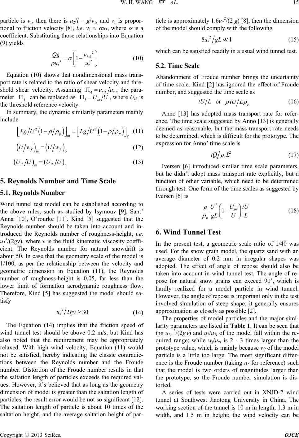

W. H. WANG ET AL.

particle is v1, then there is u2/l = g/v1, and v1 is propor-

tional to friction velocity [8], i.e. v1 ≈

u*, where

is a

coefficient. Substituting those relationships into Equation

(9) yields



= −





(10)

Equation (10) shows that nondimensional mass trans-

port rate is related to the ratio of shear velocity and thre-

shold shear velocity. Assuming

4**th

uuΠ=

, the para-

meter

can be replaced as

5th

UUΠ=

, where Uth is

the threshold reference velocity.

In summary, the dynamic similarity parameters mainly

include

( )( )

Lg ULg U

ρρ ρρ



−= −



(11)

() ( )

Uw Uw=

(12)

( )( )

th th

UU UU=

(13)

5. Reynolds Number and Time Scale

5.1. Reynolds Number

Wind tunnel test model can be established according to

the above rules, such as studied by Isymouv [9], Sant’

Anna [10], O’rourke [11]. Kind [5] suggested that the

Reynolds number should be taken into account and in-

troduced the Reynolds number of roughness-height, i.e.

u*3/(2gν), where ν is the fluid kinematic viscosity coeffi-

cient. The Reynolds number for natural snowdrift is

about 50. In case that the geometry scale of the model is

1/100, as per the relationship between the velocity and

geometric dimension in Equation (11), the Reynolds

number of roughness-height is 0.05, far less than the

lower limit of formation aerodynamic roughness flow.

Therefore, Kind [5] has suggested the model should sa-

tisfy

2 30ug

≥

(14)

The Equation (14) implies that the friction speed of

wind tunnel test should be above 0.2 m/s, but Kind has

also noted that the requirement may be appropriately

relaxed. With high wind velocity, Equation (11) would

not be satisfied, hereby indicating the classic contradic-

tions between the Reynolds number and the Froude

number. Distortion of the Froude number results in that

the saltation length of particles exceeds the required val-

ues. However, it’s believed that as long as the geometry

dimension of model is greater than the saltation length of

particles, the result error would be not so significant [12 ].

The saltation length of particle is about 10 times of the

saltation height, and the average saltation height of par-

ticle is approximately 1.6u*2/(2 g) [8], then the dimension

of the model should comply with the following

81ugL 

(15)

which can be satisfied readily in a usual wind tunnel test.

5.2. Time Scale

Abandonment of Froude number brings the uncertainty

of time scale. Kind [2] has ignored the effect of Froude

number, and suggested the time scale as

tU L

ρρ

(16)

Anno [13] has adopted mass transport rate for refer-

ence. The time scale suggested by Anno [13] is generally

deemed as reasonable, but the mass transport rate needs

to be determined, which is difficult for the prototype. The

expression for Anno’ time scale is

tQ L

(17)

Iversen [6] introduced similar time scale parameters,

but he didn’t adopt mass transport rate explicitly, but a

function of other variable, which need to be determined

through test. One form of the time scales as suggested by

Iversen [6] is

U tU

gLU L



−





(18)

6. Wind Tunnel Test

In the present test, a geometric scale ratio of 1/40 was

used. For the snow grain model, the quartz sand with an

average diameter of 0.2 mm in irregular shapes was

adopted. The effect of angle of repose should also be

taken into account in wind tunnel test. The angle of re-

pose for natural snow grains can exceed 90˚, which is

hardly realized for a model particle in wind tunnel.

However, the angle of repose is important only in the test

involved simulation of steep shape; it generally ensures

approximation as closely as possible [2].

The properties of model particles and the major simi-

larity parameters are listed in Ta ble 1. It can be seen that

the u*t 3/(2g

) and u*/u*t of the model fall within the re-

quired range; while wf/u*t is 2 - 3 times larger than the

prototype value, which is mainly because wf of the model

particle is a little too large. The most significant differ-

ence is the Froude number (taking u* for reference) such

that the model is two orders of magnitudes larger than

the prototype, so the Froude number simulation is dis-

torted.

A series of tests were carried out in XNJD-2 wind

tunnel at Southwest Jiaotong University in China. The

working section of the tunnel is 10 m in length, 1.3 m in

width, and 1.5 m in height; the wind velocity can be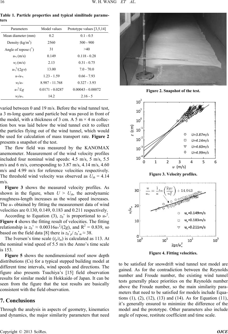

W. H. WANG ET AL.

Table 1. Particle properties and typical similitude parame-

ters

Parameters Model values Prototype values [3,5,14]

Mean diameter (mm) 0.2 0.1 - 0.5

Density (kg/m3) 2560 500 - 900

Angle of repose (˚) 31 >40

u*t (m/s) 0.149 0.118 - 0.28

wf (m/s) 2.13 0.31 - 0.75

u*t3/(2g

) 13.00 7.0 - 70.0

u*/u*t 1.23 - 1.59 0.66 - 7.93

wf/u* 8.987 - 11.768 0.327 - 3.93

u*2/Lg 0.0171 - 0.0287 0.00043 - 0.00072

wf/u*t 14.2 2.16 - 5

varied between 0 and 19 m/s. Before the wind tunn el test,

a 3 m-long qu artz sand particle bed was paved in front of

the model, with a thickness of 3 cm. A 5 m × 4 m collec-

tion box was laid below the wind tunnel exit to collect

the particles flying out of the wind tunnel, which would

be used for calculation of mass transport rate. Figure 2

presents a snapshot of the test.

The flow field was measured by the KANOMAX

anemometer. Measurement of the wind velocity profiles

included four nominal wind speeds: 4.5 m/s, 5 m/s, 5.5

m/s and 6 m/s, corresponding to 3.87 m/s, 4.14 m/s, 4.60

m/s and 4.99 m/s for reference velocities respectively.

The threshold wind velocity was observed as Uth = 4.14

m/s.

Figure 3 shows the measured velocity profiles. As

shown in the figure, when U > Uth, the aerodynamic

roughness-length increases as the wind speed increases.

The u* obtained by fitting the measurement data of wind

velocities are 0.130, 0.149, 0.183 and 0.211 respectively.

According to Equation (3), z0’ is proportional to u*2.

Figure 4 shows the fitting result of velocities. Th e fitting

relationship is z0’ ≈ 0 .00 316u*2/(2g), and R2 = 0.839, so

based on the field data [8] there is z0’p/ z0’m ≈ 38.

The Iv ersen ’s time scale (tp/tm) is calculated as 113. At

the nominal wind speed of 5.5 m/s the Anno’s time scale

is 153.

Figure 5 shows the nondimensional roof snow depth

distributions (Cs) for a typical stepped building model at

different time intervals, wind speeds and directions. The

figure also presents Tsuchiya’s [15] field observation

results for similar model in Hokkaido of Japan. It can be

seen from the figure that the test results are basically

consistent with the field observation.

7. Conclusions

Through the analysis in aspects of geometry, kinematics

and dynamics, the major similarity parameters that need

Figure 2. Snapshot of the test.

0123456

10-4

10-3

10-2

10-1

100

101

102

(m/s)

(cm)

U=3.87m /s

U=4.14m /s

U=4.60m /s

U=4.99m /s

Figure 3. Velocity profiles.

Figure 4. Fitting velocities.

to be satisfied for snowdrift wind tunnel test model are

gained. As for the contradiction between the Reynolds

number and Froude number, the existing wind tunnel

tests generally place priorities on the Reynolds number

above the Froude number, so the main similarity para-

meters that need to be satisfied for models include Equa-

tions (1), (2), (12), (13) and (14). As for Equation (11),

it’s generally ensured to minimize the difference of the

model and the prototype. Other parameters also include

angle of r e pose, restitute coefficient and time scale.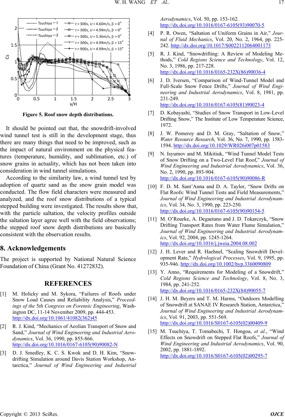

W. H. WANG ET AL.

00.5 11.5 22.5 3

0.5

1.5

x/H

Tsuchiya－1

Tsuchiya－2

Tsuchiya－3

= 300s,

= 4.60m/s,

= 0

= 300s,

= 4.99m/s,

= 0

= 300s,

= 5.36m/s,

= 0

= 300s,

= 4.99m/s,

= 15

= 900s,

= 4.99m/s,

= 15

Figure 5. Roof snow depth distr i but ions.

It should be pointed out that, the snowdrift-involved

wind tunnel test is still in the development stage, thus

there are many things that need to be improved, such as

the impact of natural environment on the physical fea-

tures (temperature, humidity, and sublimation, etc.) of

snow grains in actuality, which has not been taken into

consideration in wind tunnel simulations.

According to the similarity law, a wind tunnel test by

adoption of quartz sand as the snow grain model was

conducted. The flow field characters were measured and

analyzed, and the roof snow distributions of a typical

stepped building were investigated. The results show that,

with the particle saltation, the velocity profiles outside

the saltation layer agree well with the field observations;

the stepped roof snow depth distributions are basically

consistent with the observation results.

8. Acknowledgements

The project is supported by National Natural Science

Foundation of Chi na ( G rant No. 41 272832) .

REFERENCES

[1] M. Holicky and M. Sykora, “Failures of Roofs under

Snow Load Causes and Reliability Analysis,” Proceed-

ings of the 5th Congress on Forensic Engineering, Wash-

ington DC, 11-14 November 2009, pp. 444-453.

http://dx.doi.org/10.1061/41082(362)45

[2] R. J. Kind, “Mechanics of Aeolian Transport of Snow and

Sand,” Journal of Wind Engineering and Industrial Aero-

dynamics, Vol. 36, 1990, pp. 855-866.

http://dx.doi.org/10.1016/0167-6105(90)90082-N

[3] D. J. Smedley, K. C. S. Kwok and D. H. Kim, “Snow-

drifting Simulation around Davis Station Workshop, An-

tarctica,” Journal of Wind Engineering and Industrial

Aerodynamics, Vol. 50, pp. 153-162.

http://dx.doi.org/10.1016/0167-6105(93)90070-5

[4] P. R. Owen, “Saltation of Uniform Grains in Air,” Jour-

nal of Fluid Mechanics, Vol. 20, No. 2, 1964, pp. 225-

242. http://dx.doi.org/10.1017/S0022112064001173

[5] R. J. Kind, “Snowdrifting: A Review of Modeling Me-

thods,” Cold Regions Science and Technology, Vol. 12,

No. 3, 1986, pp. 217-228.

http://dx.doi.org/10.1016/0165-232X(86)90036-4

[6] J. D. Iversen, “Comparison of Wind-Tunnel Model and

Full-Scale Snow Fence Drifts,” Journal of Wind Engi-

neering and Industrial Aerodynamics, Vol. 8, 1981, pp.

231-249.

http://dx.doi.org/10.1016/0167-6105(81)90023-4

[7] D. Kobayashi, “Studies of Snow Transport in Low-Level

Drifting Snow,” The Institute of Low Temperature Science,

1972.

[8] J. W. Pomeroy and D. M. Gray, “Saltation of Snow,”

Water Resource Research, Vol. 36, No. 7, 19 90, pp. 1583-

1594. http://dx.doi.org/10.1029/WR026i007p01583

[9] N. Isyumov and M. Mikitiuk, “Wind Tunnel Model Tests

of Snow Drifting on a Two-Level Flat Roof,” Journal of

Wind Engineering and Industrial Aerodynamics, Vol. 36,

No. 2, 1990, pp. 893-904.

http://dx.doi.org/10.1016/0167-6105(90)90086-R

[10] F. D. M. Sant’Anna and D. A. Taylor, “Snow Drifts on

Flat Roofs: Wind Tunnel Tests and Field Measurements,”

Journal of Wind Engineering and Industrial Aerodynam-

ics, Vol. 34, No. 3, 1990, pp. 223-250.

http://dx.doi.org/10.1016/0167-6105(90)90154-5

[11] M. O’Rourke, A. Degaetano and J. D. Tokarczyk, “Snow

Drifting Transport Rates from Water Flume Simulation,”

Journal of Wind Engineering and Industrial Aerodynam-

ics, Vol. 92, 2004, pp. 1245-1264.

http://dx.doi.org/10.1016/j.jweia.2004.08.002

[12] J. H. Lever and R. Haehnel, “Scaling Snowdrift Devel-

opment Rate,” Hydrological Processes, Vol. 9, 1995, pp.

935-946. http://dx.doi.org/10.1002/hyp.3360090809

[13] Y. Anno, “Requirements for Modeling of a Snowdrift,”

Cold Regions Science and Technology, Vol. 8, No. 3,

1984, pp. 241-252.

http://dx.doi.org/10.1016/0165-232X(84)90055-7

[14] J. H. M. Beyers and T. M. Harms, “Outdoors Modelling

of Snowdrift at SANAE IV Research Station, Antarctica,”

Journal of Wind Engineering and Industrial Aerodynam-

ics, Vol. 91, 2003, pp. 551-569.

http://dx.doi.org/10.1016/S0167-6105(02)00409-9

[15] M. Tsuchiya, T. Tomabechi, T. Hongoa, et al., “Wind

Effects on Snowdrift on Stepped Flat Roofs,” Journal of

Wind Engineering and Industrial Aerodynamics, Vol. 90,

2002, pp. 1881-1892.

http://dx.doi.org/10.1016/S0167-6105(02)00295-7