Application of ESMD Method to Air-Sea Flux Investigation

doi:10.4236/ijg.2013.45B002

Paper Menu >>

Journal Menu >>

International Journal of Geosciences, 2013, 4, 8-11

http://dx.doi.org/10.4236/ijg.2013.45B002 Published Online September 2013 (http://www.scirp.org/journal/ijg)

Application of ESMD Method to Air-Sea Flux I n ves tigation

Hui-Feng Li, Jin-Liang Wang*, Zong-Jun Li

College of Science, Qingdao Technological University, East Jialingjiang Road No. 777,

Huangdao Region of Qingdao, China

Email: *[email protected]

Received May 2013

ABSTRACT

The ESMD method can be seen as a new alternate of the well-known Hilbert-Huang transform (HHT) for non-steady

data processing. It is good at finding the optimal adaptive global mean fitting curve, which is superior to the common

least-square method and running-mean approach. Take the air-sea momentum flux investigation as an example, only

when the non-turbulent wind components is well extracted, can the remainder signal be seen as actual oscillations

caused by turbulence. With the aid of −5/3 power law for the turbulence, a mode-filtering approach based on ESMD

decomposition is developed here. The test on observational data indicates that this approach is very feasible and it may

greatly reduce the error caused by the non-turbulent components.

Keywords: Extreme-Point Symmetric Mode Decomposition (ESMD); Air-Sea Flux; Hilbert-Huang Transform (HHT );

Fourier Frequency Spectrum; Empirical Mode Decomposition (EMD); Wind; Momentum Flux

1. Introduction

The ESMD method is the abbreviation of “extreme-point

symmetric mode decomposition” method [1] which can

be seen as a new alternate of the well-known Hilbert-

Huang transform (HHT) method [2], and it is anticipated

as an effective usage in the fields of atmospheric and

oceanic sciences, informatics, economics, ecology, med-

icine and seismology etc. Now the corresponding paper

is available at http://arxiv.org/abs/1303.6540 with a pro-

tection of software by the national copyright administra-

tion of Chi na [3,4].

Historically, in the field of data processing there are

three typical methods: (1) The classical Fourier transform

method, it is suitable for linear and stationary data; (2)

The popular Wavelet transform method, it is suitable for

linear and non-stationary data; (3) The hot HHT method

based on the empirical mode decomposition (EMD), it is

suitable for nonlinear and non-stationary data. At present,

HHT is the most advanced method and is widely used.

But there are also some shortcomings in it, such as: a)

How to choose the stoppage criteria is a puzzling prob-

lem [5]; b) The residual component is too rough to reflect

the whole evolutionary trend; c) The Hilbert-spectrum

analyzing approach has some inherent defects.

Our ESMD method has not only remedied the short-

comings of HHT but also developed several new features

as follows: (1) the outer envelop interpolation is changed

to the inner extreme-point symmetr ic one; (2) the resi-

dual component is optimized by the sifting times; (3) in

view of the defect of all the integral transforms in time-

frequency analysis, the tradit ional approach is abandoned

and a data-based “direct interpolating” one is developed.

For a given data, its frequency analysis should be done

on the oscillating part. Hence, to clear away the global

mean curve is the first and foremost problem. In fact,

only when the global mean curve is an optimal one, can

the remainder signal be seen as actual oscillations cause d

by a series of wave fluctuations. In this sense, the ESMD

method also offers a good adaptive approach for finding

the optimal global mean fitting curve. It is superior to the

commonly used least-square method (requires a priori

function form) and running-mean approach (lacks of

theoretical base and different choices of time-window

and weight coefficients may result in different curves).

This advantage is good for air-sea flux investigation.

2. On the Air-Sea Flux

The importance of air-sea interaction to the earth’s cli-

mate is widely appreciated and this attracts the research-

ers to make more in situ flux observations at sea. Among

all the air-sea flux measurement methods, the commonly

used are the direct eddy-covariance method [6] and the

inertial-dissipation method [7,8]. The first one is based

on the initial definition of the flux, which performs well

on fixed platforms and it requires velocity corrections in

case the platform is a moving one [9-14]. The second one

is based on the inertial-dissipation arguments of the tur-

*Corresponding a uthor.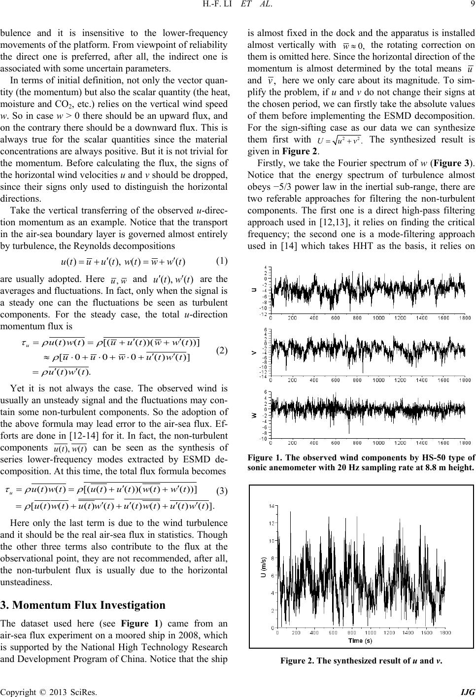

H.-F. LI ET AL.

bulence and it is insensitive to the lower-frequency

movements of the platform. From viewpoint of reliability

the direct one is preferred, after all, the indirect one is

associated with some uncertain parameters.

In terms of initial definition, n ot only the vector qua n-

tity (the momentum) but also the sca lar quantity (the heat,

moisture and CO2, etc.) relies on the vertical wind speed

w. So in case w > 0 there should be an upward flux, and

on the contrary there should be a downward flux. This is

always true for the scalar quantities since the material

concentrations are always positive. But it is not trivial for

the momentum. Before calculating the flux, the signs of

the horizontal wind v elocities u and v should be dropped,

since their signs only used to distinguish the horizontal

directions.

Take the vertical transferring of the observed u-direc-

tion momentum as an example. Notice that the transport

in the air-sea boundary layer is governed almost entirely

by turbul e nc e, the Reynolds decompositi ons

()(), ()()utuutwtww t

′′

=+=+

(1)

are usually adopted. Here

,uw

and

(), ()ut wt

′′

are the

averages and fluctuations. In fact, only when the signal is

a steady one can the fluctuations be seen as turbulent

components. For the steady case, the total u-direction

momentum flux is

( )( )[(( ))(( ))]

[000()()]

()().

utwtuutww t

uuwutwt

utwt

τρ ρ

′′

= =++

′′

≈⋅+ ⋅+⋅+

′′

(2)

Yet it is not always the case. The observed wind is

usually an unsteady signal and the fluctuations may con-

tain some non-turbulent components. So the adoption of

the above formula may lead error to the air-sea flux. Ef-

forts are done in [12-14] for it. In fact, the non-turbulent

components

(), ()ut wt

can be seen as the synthesis of

series lower-frequency modes extracted by ESMD de-

composition. At this time, the total flux formula becomes

()()[(()())(()())]

[() ()()()()()()()].

utwtutu twtw t

utwt utwt utwt utwt

τρ ρ

′′

==++

′ ′′′

= +++

(3)

Here only the last term is due to the wind turbulence

and it should be the real air-sea flux in statistics . Though

the other three terms also contribute to the flux at the

observational point, they are not recommended, after all,

the non-turbulent flux is usually due to the horizontal

unsteadiness.

3. Momentum Flux Investigation

The dataset used here (see Figure 1) came from an

air-sea flux experiment on a moored ship in 2008, which

is supported by the National High Technology Research

and Development Program of China. Notice that the ship

is almost fixed in the dock and the apparatus is installed

almost vertically with

0,w≈

the rotating correction on

them is omitted her e. Since the horizontal direction of the

momentum is almost determined by the total means

and

here we only care about its magnitude. To sim-

plify the problem, if u and v do not change their signs at

the chosen period, we can firstly take the absolute values

of them before implementing the ESMD decomposition.

For the sign-sifting case as our data we can synthesize

them first with

.U uv= +

The synthesized result is

given in Figu re 2.

Firstly, we take the Fourier spectrum of w (Figure 3).

Notice that the energy spectrum of turbulence almost

obeys −5/3 power law in the inertial sub-range, there are

two referable approaches for filtering the non-turbulent

components. The first one is a direct high-pass filtering

approach used in [12,13], it relies on finding the critical

frequency; the second one is a mode-filtering approach

used in [14] which takes HHT as the basis, it relies on

Figure 1. The observed wind components by HS-50 type of

sonic anemometer with 20 Hz sampling rate at 8.8 m height.

Figure 2. The synthesized resul t of u and v.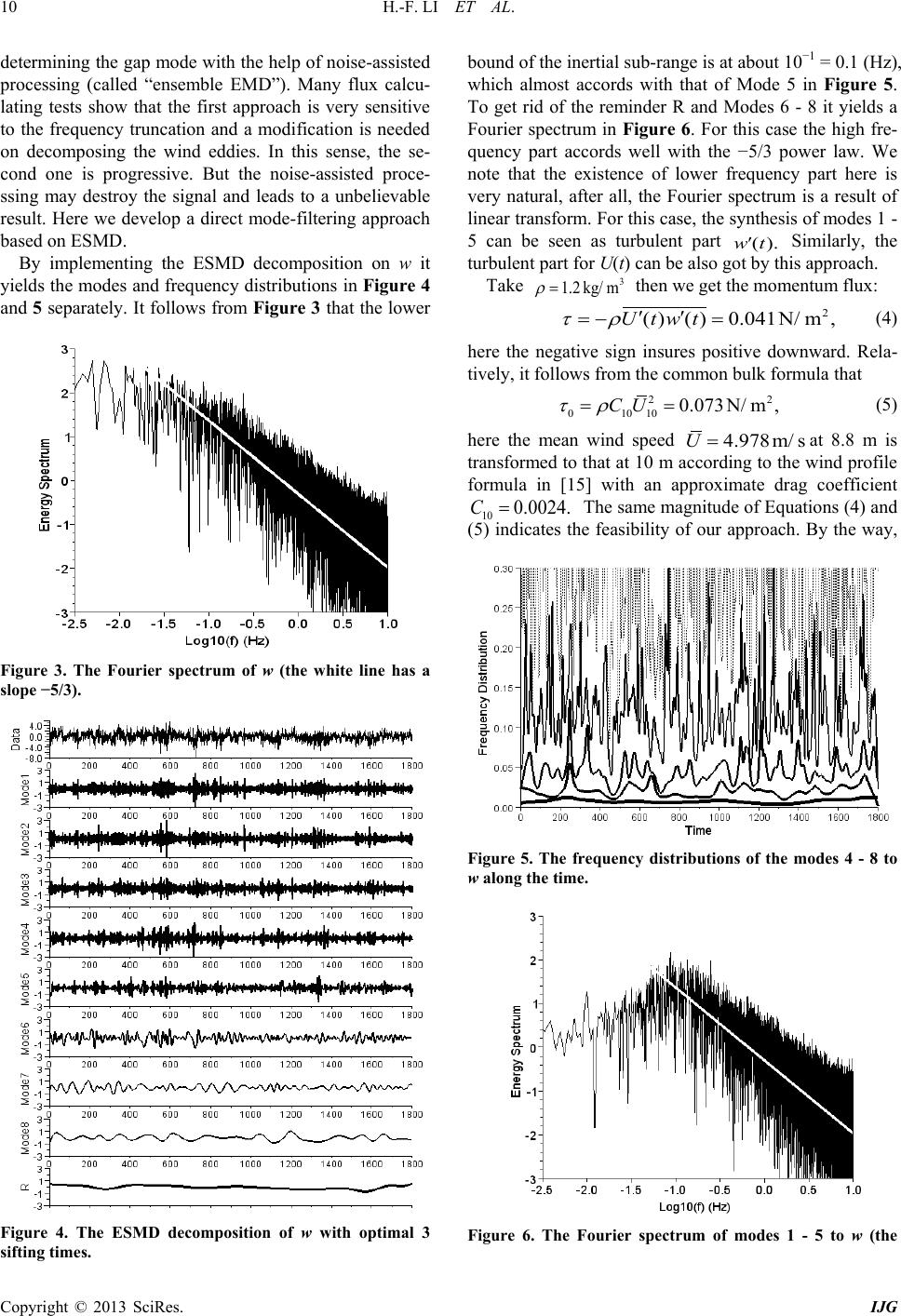

H.-F. LI ET AL.

determining the gap mode with the help of noise-assisted

processing (called “ensemble EMD”). Many flux calcu-

lating tests show that the first approach is very sensitive

to the frequency truncation and a modification is needed

on decomposing the wind eddies. In this sense, the se-

cond one is progressive. But the noise-assisted proce-

ssing may destroy the signal and leads to a unbelievable

result. Here we develop a direct mode-filtering approach

based on ESMD.

By implementing the ESMD decomposition on w it

yields the modes and frequency distributions in Figure 4

and 5 separately. It follows from Figure 3 that the lower

Figure 3. The Fourier spectrum of w (the white line has a

slope −5/3).

Figure 4. The ESMD decomposition of w with optimal 3

sifting times.

bound of the inertia l su b-range is at abou t 10 −1 = 0.1 (Hz),

which almost accords with that of Mode 5 in Figure 5.

To get rid of the reminder R and Modes 6 - 8 it yields a

Fourier spectrum in Figure 6. For this case the high fre-

quency part accords well with the −5/3 power law. We

note that the existence of lower frequency part here is

very natural, after all, the Fourier spectrum is a result of

linear transform. For this case, the synthesis of modes 1 -

5 can be seen as turbulent part

( ).wt

′

Similarly, the

turbulent part for U(t) can be a lso got by this approac h.

Take

1.2 kg/ m

then we get the momentum flux:

( )( )0.041N/m,U twt

τρ

′′

=−=

(4)

here the negative sign insures positive downward. Rela-

tively, it follows from the common bulk formula that

010 100.073N/ m,CU

τρ

= =

(5)

here the mean wind speed

4.978m/ sU=

at 8.8 m is

transformed to that at 10 m according to the wind profile

formula in [15] with an approximate drag coefficient

0.0024.C=

The same magnitude of Equations (4) a nd

(5) indicates the feasibility of our approach. By the way,

Figure 5. The frequency distributions of the modes 4 - 8 to

w along the time.

Figure 6. The Fourier spectrum of modes 1 - 5 to w (the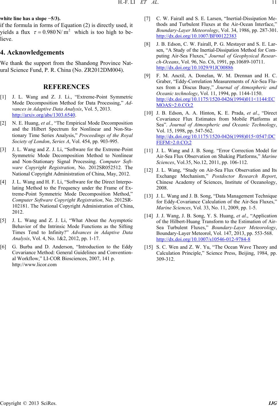

H.-F. LI ET AL.

white line has a slope −5/3).

if the formula in forms of Equation (2) is directly used, it

yields a flux

0.980N/ m

which is too high to be-

lieve.

4. Acknowledgements

We thank the support from the Shandong Province Nat-

ural Science Fund, P. R. China (No . ZR2012 DM004) .

REFERENCES

[1] J. L. Wang and Z. J. Li., “Extreme-Point Symmetric

Mode Decomposition Method for Data Processing,” Ad-

vances in Adaptive Data Analysis, Vol. 5, 2013.

http://arxiv.org/abs/1303.6540.

[2] N. E. Huang, et al., “The Empirical Mode Decomposition

and the Hilbert Spectrum for Nonlinear and Non-Sta-

tionary Time Series Analysis,” Proceedings of the Royal

Society of London, Series A, Vol. 454, pp. 903-995.

[3] J. L. Wang and Z. J. Li, “Software for the Extreme-Point

Symmetric Mode Decomposition Method to Nonlinear

and Non-Stationary Signal Processing. Computer Soft-

ware Copyright Registration, No. 2012SR052512. The

[4] J. L. Wang and H. F. Li, “Software for the Direct Interpo-

lating Method to the Frequency under the Frame of Ex-

treme-Point Symmetric Mode Decomposition Method,”

Computer Software Copyright Registration, No. 2012SR-

102181. The National Copyright Administration of China,

2012.

[5] J. L. Wang and Z. J. Li, “What About the Asymptotic

Behavior of the Intrinsic Mode Functions as the Sifting

Times Tend to Infinity?” Advances in Adaptive Data

Analysis, Vol. 4, No. 1&2, 2012, pp. 1-17.

[6] G. Burba and D. Anderson, “Introduction to the Eddy

Covariance Method: General Guidelines and Convention-

al Workflow,” LI-COR Biosciences, 2007, 141 p.

http://www.licor.com

[7] C. W. Fairall and S. E. Larsen, “Inertial-Dissipation Me-

thods and Turbulent Fluxes at the Air-Ocean Interface,”

Boundary-Layer Meteorology, Vol. 34, 1986, pp. 287-301.

http://dx.doi.org/10.1007/BF00122383

[8] J. B. Edson, C. W. Fairall, P. G. Mestayer and S. E. Lar-

sen, “A Study of the Inertial-Dissipation Method for Com-

puting Air-Sea Fluxes,” Journal of Geophysical Resear-

ch-Oceans, Vol. 96, No. C6, 1991, pp.10689-10711.

http://dx.doi.org/10.1029/91JC00886

[9] F. M. Anctil, A. Donelan, W. M. Drennan and H. C.

Graber, “Eddy-Correlation Measurements of Air-Sea Flu-

xes from a Discus Buoy,” Journal of Atmospheric and

Oceanic technology, Vol. 11, 1994, pp. 1144-1150.

http://dx.doi.org/10.1175/1520-0426(1994)011<1144:EC

MOAS>2.0.CO;2

[10] J. B. Edson, A. A. Hinton, K. E. Prada, et al., “Direct

Covariance Flux Estimates from Mobile Platforms at

Sea”. Journal of Atmospheric and Oceanic Technology,

Vol. 15, 1998, pp. 547-562.

http://dx.doi.org/10.1175/1520-0426(1998)015<0547:DC

FEFM>2.0.CO;2

[11] J. L. Wang and J. B. Song. “Error Correction Model for

Air-Sea Flux Observation on Shaking Platforms,” Marine

Sciences, Vol.35, No.12, 2011, pp. 106-112.

[12] J. L. Wang, “Study on Air-Sea Flux Observation and Its

Exchange Mechanism,” Postdoctor Research Report,

Chinese Academy of Sciences, Institute of Oceanology,

2008.

[13] J. L. Wang and J. B. Song, “Data Management Technique

for Eddy-Covariance Calculation of the Air-Sea Fluxes,”

Marine Sciences, Vol. 33, No. 11, 2009, pp. 1-5.

[14] J. J. Wang, J. B. Song, Y. S. Huang, et al., “Application

of the Hilbert-Huang Transform t o the Estimation of Air -

Sea Turbulent Fluxes,” Boundary-Layer Meteorology,

Boundary-Layer Meteorol, Vol. 147, 2013, pp. 553-568.

http://dx.doi.org/10.1007/s10546-012-9784-8

[15] S. C. Wen and Z. W. Yu, “The Ocean Wave Theory and

Calculation Principle,” Science Press, Beijing, 1984, pp.

309-312.