Least Action Trajectory in Neural Networks

doi:10.4236/ojapps.2013.33B002

Paper Menu >>

Journal Menu >>

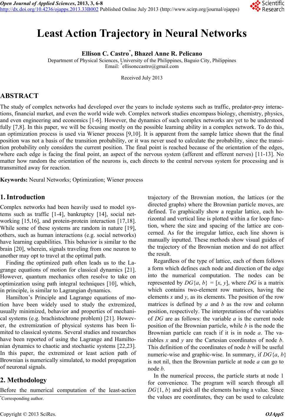Open Journal of Applied Sciences, 2013, 3, 6-8

http://dx.doi.org/10.4236/ojapps.2013.33B002 Published Online July 2013 (http://www.scirp.org/journal/ojapps)

Least Action Trajectory in Neural Networks

Ellison C. Castro*, Bhazel Anne R. Pelicano

Department of Physical Sciences, University of the Philippines, Baguio City, Philippines

Email: *[email protected]

Received July 2013

ABSTRACT

The study of complex networks had developed over the years to include systems such as traffic, predator-prey interac-

tions, financial market, and even the world wide web. Complex network studies encompass biology, chemistry, physics,

and even engineering and economics [1-6]. However, the dynamics of such complex networks are yet to be understood

fully [7,8]. In this paper, we will be focusing mostly on the po ssible learning ability in a complex network. To do this ,

an optimization process is used via Wiener process [9,10]. It is apparent from the sample lattice shown that the final

position was not a basis of the transition probability, or it was never used to calculate the probability, since the transi-

tion probability only considers the current position. The final point is reached because of the orientation of the edges,

where each edge is facing the final point, an aspect of the nervous system (afferent and efferent nerves) [11-13]. No

matter how random the orientation of the neurons is, each directs to the central nervous system for processing and is

transmitted away for reaction.

Keywords: Neura l Ne t works; Optimization; Wiene r process

1. Introduction

Complex networks had been heavily used to model sys-

tems such as traffic [1-4], bankruptcy [14], social net-

working [15,16], and protein-protein interaction [17,18].

While some of these systems are random in nature [19],

others, such as human interactions (e.g. social networks)

have learning capabilities. This behavior is similar to the

brain [20], wherein, signals traveling from one neuron to

another may opt to travel at the optimal path.

Finding the optimized path often leads us to the La-

grange equations of motion for classical dynamics [21].

However, quantum mechanics often resolve to take on

optimization using path integral techniques [10], which,

in principle, is simil a r to La g rangian dynamic s .

Hamilton’s Principle and Lagrange equations of mo-

tion have been widely used to study the extremized,

usually minimized, behavior and properties of mechani-

cal systems (e.g. brachistochrone problem) [21]. Howev-

er, the extremization of physical systems has been li-

mited to classical systems. Several studies and researches

have been reported of using the Lagrange and Hamilto-

nian dynamics to chaotic and stochastic systems [22 ,23].

In this paper, the extremized or least action path of

Brownian is numerically simulated, to model propagation

of neuronal signals.

2. Methodology

Before the numerical computation of the least-action

trajectory of the Brownian motion, the lattices (or the

directed graphs) where the Brownian particle moves, are

defined. To graphically show a regular lattice, each ho-

rizontal and vertical line is plotted within a for loop f un c-

tion, where the size and spacing of the lattice are con-

cerned. As for the irregular lattice, each line shown is

manually inputted. These methods show visual guides of

the trajectory of the Brownian motion and do not affect

the result.

Regardless of the type of lattice, each of them follows

a form which defines each node and direction of the edge

into the numerical computation. The nodes can be

represented by DG{a, b} = [x, y], where DG is a matrix

which contains two-element row matrices, having the

elements x and y, as its elements. The position of the row

matrices is defined by a and b as the row and column

position, respectively. The in terpretation s of the variab les

of DG are as follows: the variable a is the current node

position of th e Brownian particle, while b is the node the

Brownian particle can reach if it is in node a. The va-

riables x and y are the Cartesian coordinates of node b.

This definition of the coordinates of node b will be useful

numeric-wise and graphic-wise. In summary, if DG{a, b}

is not nil, then the Brownian particle at node a can go to

node b.

In the numerical process, the particle starts at node 1

for convenience. The program will search through all

DG{1, b} and pick all the elements having a value. Since

the values are coordinates, they can be used to calculate

Corresponding author.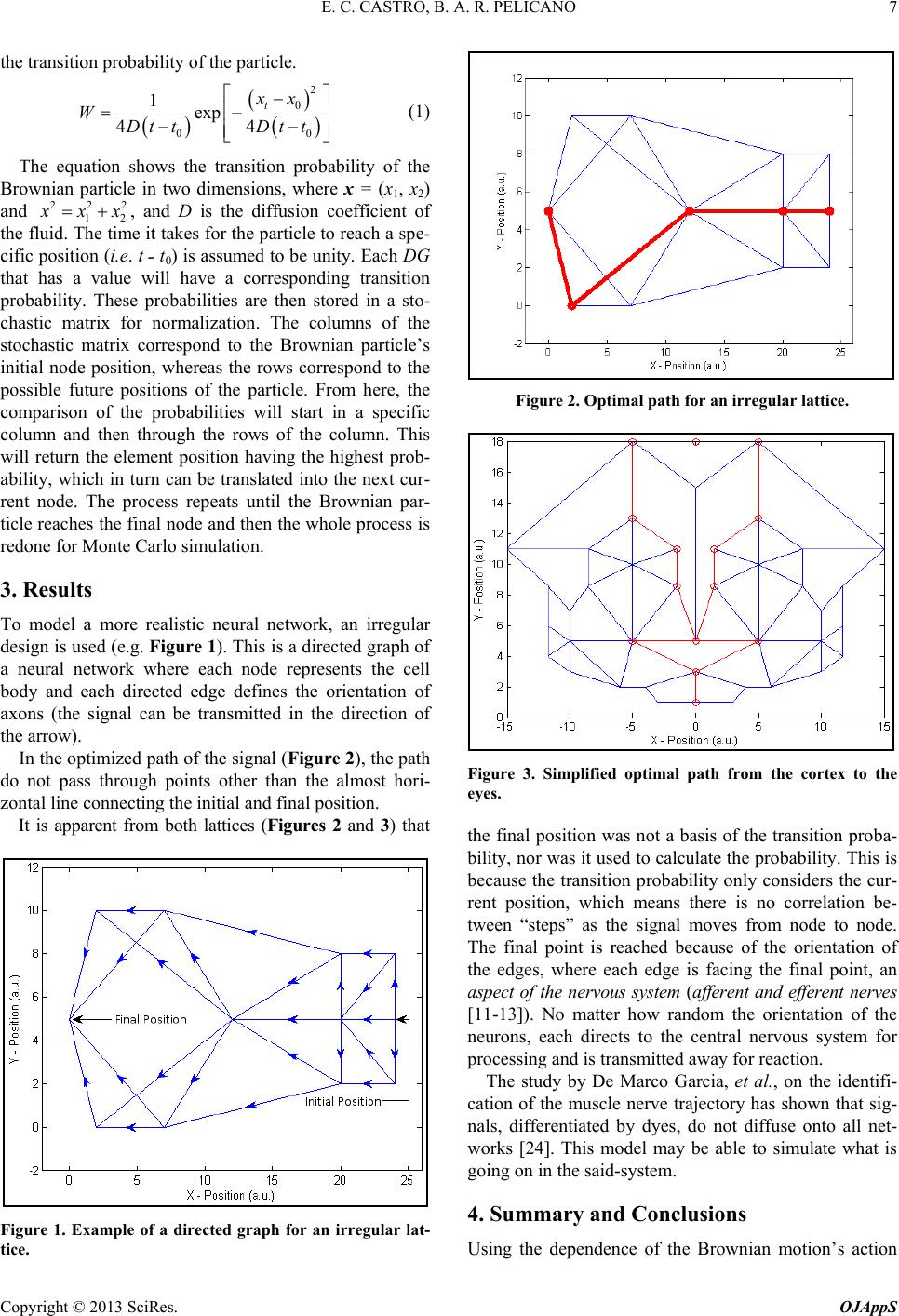

E. C. CASTRO, B. A. R. PELI CANO

the transition probability of the particle.

( )

1exp

WDt tDt t



−

= −



−−





(1)

The equation shows the transition probability of the

Brownian particle in two dimensions, where x = (x1, x2)

and

2 22

xxx= +

, and D is the diffusion coefficient of

the fluid. The time it takes for the particle to reach a spe-

cific position (i.e. t ˗ t0) is assumed to be unity. Each DG

that has a value will have a corresponding transition

probability. These probabilities are then stored in a sto-

chastic matrix for normalization. The columns of the

stochastic matrix correspond to the Brownian particle’s

initial node position, whereas the rows correspond to the

possible future positions of the particle. From here, the

comparison of the probabilities will start in a specific

column and then through the rows of the column. This

will return the element position having the highest prob-

ability, which in turn can be translated into the next cur-

rent node. The process repeats until the Brownian par-

ticle reaches the final node and then the whole process is

redone for Monte Carlo simulation.

3. Results

To model a more realistic neural network, an irregular

design is used (e.g. Figure 1). This is a directed graph of

a neural network where each node represents the cell

body and each directed edge defines the orientation of

axons (the signal can be transmitted in the direction of

the arrow).

In the optimized path of the signal (Figure 2), the path

do not pass through points other than the almost hori-

zontal line connecting the initial and fina l position.

It is apparent from both lattices (Figures 2 and 3) that

Figure 1. Example of a directed graph for an irregular lat-

tice.

Figure 2. Optimal path for an irregular lattice.

Figure 3. Simplified optimal path from the cortex to the

eyes.

the final position was not a basis of the transition proba-

bility, nor was it used to calculate the probability. This is

because the transition probability only considers the cur-

rent position, which means there is no correlation be-

tween “steps” as the signal moves from node to node.

The final point is reached because of the orientation of

the edges, where each edge is facing the final point, an

aspect of the nervous system (afferent and efferent nerves

[11-13]). No matter how random the orientation of the

neurons, each directs to the central nervous system for

processing and is transmitted away for reaction.

The study by De Marco Garcia, et al., on the identifi-

cation of the muscle nerve trajectory has shown that sig-

nals, differentiated by dyes, do not diffuse onto all net-

works [24]. This model may be able to simulate what is

going on in the said-system.

4. Summary and Conclusions

Using the dependence of the Brownian motion’s action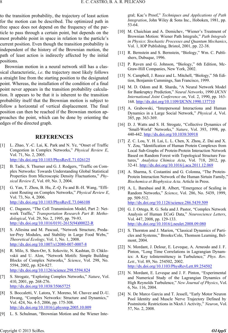

E. C. CASTRO, B. A. R. PELI CANO

to the transition probability, the trajectory of least action

for the motion can be described. The optimized path in

free space does not depend on the frequency of the par-

ticle to pass through a certain point, but depends on the

most probable point in space in relation to the particle’s

current position. Even though the transition probability is

independent of the history of the Brownian motion, the

path of least action is indirectly affected by the initial

positions.

Brownian motion in a neural network still has a clas-

sical characteristic, i.e. the trajectory most likely follows

a straight line fro m the starting position to the d esignated

point. Whereas, the installation of the cond ition of a final

point never appears in the transition probability calcula-

tion. It appears to be that it is inherent to the transition

probability itself that the Brownian motion is subject to

follow a horizontal of vertical displacement. The final

position can then be reached if the Brownian motion ap-

proaches the point, which can be done by orienting the

edges of t he directed graph.

REFERENCES

[1] L. Zhao, Y.-C. Lai, K. Park and N. Ye, “Onset of Traffic

Congestion in Complex Networks,” Physical Review E,

Vol. 71, No. 2, 2005.

http://dx.doi.org/10.1103/PhysRevE.71.026125

[2] B. Tadic, S. Thurner and G. J. Rodgers, “Traffic on Com-

plex Networks: Towards Understanding Global Statistical

Properties from Microscopic Density Fluctuations,” Phy -

sical Review E , Vol. 69, No. 3, 2004.

[3] G. Yan, T. Zhou, B. Hu , Z.-Q. Fu and B.-H. Wang , “Effi-

cient Routing on Complex Networks,” Physical Review E,

Vol. 73, No. 4, 2006.

http://dx.doi.org/10.1103/PhysRevE.73.046108

[4] C. Daganzo, “The Cell Transmission Model, Part 2: Net-

work Traffic,” Transportation Research Part B: Metho-

dological, Vol. 29, No. 2, 1995, pp. 79-93.

http://dx.doi.org/10.1016/0191-2615(94)00022-R

[5] S. Allesina and M. Pascual, “Network Structure, Preda-

tor-Prey Modules, and Stability in Large Food Webs,”

Theoretical Ecology, Vol. 1, No. 1, 2008.

http://dx.doi.org/10.1007/s12080-007-0007-8

[6] R. Milo, S. Shen-Orr, S. It zkovitz, N. Kashtan, D. Chklo-

vskii and U. Alon, “Network Motifs: Simple Building

Blocks of Complex Networks,” Scienc e , Vol. 298, No.

5594, 2002, pp. 824-827.

http://dx.doi.org/10.1126/science.298.5594.824

[7] S. Strogatz, “Exploring Complex Networks,” Nature, Vol.

410, 2001, pp. 268-276.

http://dx.doi.org/10.1038/35065725

[8] S. Boccaletti, V. Latora, Y. Moreno, M. Chavez and D.-U.

Hwang, “Complex Networks: Structure and Dynamics,”

Vol. 424, No. 4-5, 2006, pp. 175-308.

http://dx.doi.org/10.1016/j.physrep.2005.10.009

[9] L. S. Schulman, “Brownian Motion and the Wiener Inte-

gral; Kac’s Proof,” Techniques and Applications of Path

Integration, John Wiley & Sons Inc., Hoboken, 1981, pp.

53-64.

[10] M. Chaichian and A. Demichev, “Wiener’s Treatment of

Brownian Motion: Wiener Path Integrals,” Path Integrals

in Physics: Stochastic Processes and Quantum Mechanics,

Vol. 1, IOP Publishing, Bristol, 2001, pp. 22-38.

[11] R. Bernstein and S. Bernstein, “Biology,” Wm. C. Publi-

shers, Dubuque, 1996.

[12] P. Raven and G. Johnson, “Biology,” 6th Edition, Mc-

Graw-Hill Companies, New York, 2002.

[13] N. Campbell, J. Reece and L. Mitchell, “Biology,” 5th Edi-

tion, Benjamin Cummings, San Francisco, 1999.

[14] M. D. Odom and R. Sharda, “A Neural Network Model

for Bankruptcy Prediction,” Neural Network s, 1990 IJCNN

International Joint Conference on, Vol. 2, 1990, pp. 163-

168. http://dx.doi.org/10.1109/IJCNN.1990.137710

[15] A. Grabowski, “Interpersonal Interactiona and Human

Dynamics in a Large Social Network,” Physical A, Vol.

385, pp. 363-369.

[16] D. J. Watts and S. H. Strogatz, “Collective Dynamics of

‘Small-World’ Networks,” Nature, Vol. 393, 1998, pp.

440-442. http://dx.doi.org/10.1038/30918

[17] Z. C. Lou, Y. H. Lai, L. L. Chen, X. Zhou, Z. Dai and X.

Y. Zou, “Identific ation of Human Protein Complexes from

Local Sub-Graphs of Protein-Protein Interaction Network

Based on Random Forest with Topological Structure Fea-

tures,” Analytica Chimica Acta, Vol. 718, 2012, pp.

32-41. http://dx.doi.org/10.1016/j.aca.2011.12.069

[18] A. Sharma, S. Costantini and G. Colonna, “The Protein-

Protein Interaction Network of the Human Sirtuin Family,”

Biochemica et Biophysica Acta. Article in Press.

[19] A. L. Barabasi and R. Albert, “Emergence of Scaling in

Random Networks,” Science, Vol. 286, No. 5439, 1999,

pp. 509-512.

http://dx.doi.org/10.1126/science.286.5439.509

[20] G. J. Ortega, R. G. Sola and J. Pastor, “Complex Network

Analysis of Human ECoG Data,” Neuroscience Letters,

Vol. 447, 2008, pp. 129-133.

http://dx.doi.org/10.1016/j.neulet.2008.09.080

[21] S. Thornton and J. Marion, “Classical Dynamics of Parti-

cles and Systems,” Brooks/Cole, Thomson Learning, Bel -

mont, 2004.

[22] N. Mordant, J. De lour, E. Leveque, A. Arneodo and J. F.

Pinton, “Long Time Correlations in Lagrangian Dynam-

ics: A Key toIntermittency in Turbulence,” Phys. Rev.

Lett., Vol. 89, No. 254502, 2002.

http://dx.doi.org/10.1103/PhysRevLett.89.254502

[23] N. Mordant, E. Leveque and J. F. Pinton, “Experimental

and Numerical Study of the Lagrangian Dynamics of

High Reynolds Turbulence,” New Journal of Physics, Vol.

6, No. 116, 2004.

[24] N. De Marco Garcia and T. Jessell, “Early Motor Neuron

Pool Identity and Muscle Nerve Trajectory Defined by

Postmitotic Restrictions in Nkx6.1 Activity ,” Neuron , Vol.

57, No. 2, 2008.