High-Impedance Bus Differential Protection Modeling in ATP/MODELS

doi:10.4236/eng.2013.59B007

Paper Menu >>

Journal Menu >>

Engineering, 2013, 5, 37-42

http://dx.doi.org/10.4236/eng.2013.59B007 Published Online September 2013 (http://www.scirp.org/journal/eng)

High-Impedance Bus Differential Protection Modeling

in ATP/MODELS

Mardênnia T. S. Alvarenga, Priscila L. Vianna, Kleber M. Silva

Power System Protection Labora t ory, Departmen t of E lectrical En gi ne ering, University of Brasilia, Brasilia, Brazil

Email: [email protected]

Received July 2013

Abstract

This paper presents a modeling of a high-impedance bus differential protection logic using the ATP (Alternative Tran-

sients Program) MODELS language. The model is validated using ATP simulations on an electrical system consisting

of a sectionalized bus arrangement with four transmission lines (TLs) and two autotransformers. The obtained results

validate the model and present some of the advantages of using this type of bus protection, such as fast and safe opera-

tion, even when under adverse conditions such as current transformers (CTs) magnetic core saturation upon the occur-

rence of external faults.

Keywords: Bus Protection; High-Impedance Differential Protection; ATP; MODELS

1. Introduction

The increasing demand for energy supplies and lower

fares cause the electricity sector to operate close to its

stability limits, which may compromise the safety of its

operation. In this context, the protection of electric power

system plays a key role in order to extinguish system

faults quickly and appropriately, preserving the integrity

of the system components, avoiding blackouts of major

proportions and preserving load as much as possible.

Among faults in electric apparatus, sub station (S E ) bus

deserves serious attention. Even though faults in these

components are not very common—about 5%— [1], its

effects are very harmful to the system, and can often lead

it to instability.

With respect to the station-bus protection, two tech-

niques are widely used: low impedance differential pro-

tection and high-impedance differential protection. The

second one is typically used in SEs with rated voltage

greater or equal to 500 kV, where buses have arrange-

ments with fixed topology and there are less occurrences

of switching mane uvers in CTs secondar y circuits.

Softwares traditionally used for analysis of protection

systems use component models dedicated to the analysis

of the power system at fundamental frequency. As a re-

sult, the transient performances of the protection systems

are not evaluated. In this way, EMTP (Eletromagnetic

Transient Programs) softwares have shown to be an ap-

propriate alternative for modeling and simulating protec-

tive relays, since they use more thorough models of the

sys te m co mponents and provide suitable environments to

link user -defined numeric relays models.

In the state-of-art of relay modeling in EMTP software,

most papers on the subject deal with the transmission

lines (TL) distance protection [2-5]. In [2], a distance

relay is modeled in EMTP program and its performance

is compared with the one of a manufactured relay. In [3]

and [4], distance protection schemes applied to three

terminals line and double circuit lines are evaluated, re-

spectively. In both researches, the relay is modeled with

the use of MODELS language of ATP. In [5], a Visual

C++ based program is implemented to obtain the FOR-

TRAN code that represents the functional blocks of the

relay, which is incorporated in a PSCAD/EMTDC simu-

lation.

To the authors’ best knowledge, there are no papers in

the state-of-art that present high-impedance bus differen-

tial protection modeling and simulation in EMTP soft-

wares, which became the motivation and objective for the

development of this paper: propose, implement and vali-

date a high-impedance bus differential protection model in

ATP for use in power system protection schemes analysis.

The proposed model of the numerical differential pro-

tection was done using MODELS language of ATP and

can be divided into four modules: signal condition, data

acquisition, phasor estimation and differential analysis.

The first one implements the model of an anti-aliasing

analog filter. The second one implements the models of

the Sample/Holder and A/D Converter. In the third mod-

ule, the phasor’s amplitude and argument are calculated

in the fundamental frequency. Finally, the high-impedance

bus differential protection logic is implemented in the

M. T. S. ALVARENGA ET AL.

fourth and last module.

The model is validated using ATP simulations on an

electrical system consisting of a sectionalized bus ar-

rangement with four transmission lines (TLs) and two

autotransformers. The obtained results validate the model

and present some of the advantages of using this type of

bus protection.

2. Fundamentals of High -Impedance Bus

Differential Protection

In order to understand the systematic of high-impedance

bus differential protection, a single bus arrangement with

four transmission lines will be used (Figure 1).

To accomplish the differential protection closed loop,

the physical parallel connection of the CTs secondary is

necessary, as shown in Figure 1. The connected CTs

must have the same ratio in order to minimize the differ-

ence in performance between them.

As shown in Figure 1, the high-impedance bus diffe-

rential relay inter nal elements are applied to the common

node of all CTs. Rsis the stabilizing resistance, which

has typical value of 2000 Ω, and determines the high-

impedance input of the relay.

The 87Z element is a sensitive, low-impedance, ad-

justable pick-up current element scaled in voltage [6].

Since the branch current formed by these two compo-

nents is low, the high-impedance bus differential relay

trip becomes dependent on voltage in its terminals.

The Metal Oxide Varistor (MO V ) is a non-linear re-

sistance connected across the high-impedance circuit to

prevent high voltage from damaging the relay and CT

circuitry [6] .

The instantaneous overcurrent relay (50) and timed

overcurrent relays (51) control the breaker opening, dur-

ing abnormal conditions of operation of the system

which cause high current magnitudes.

The high-impedance relay is set to trip based on the

relay pickup thr eshold

( )

pick up

−

. This value must be set

Figure 1. Example of high-impedance bus diff erential relay

schematic.

above the highest voltage measurement across the relay

with a completely saturated CT for external faults cond i-

tions. This ensures safety for external-fault protection.

2.1. Normal Conditions and External Faults

without CT Saturation

In Fi gure 2, CT A represents the parallel combination of

the CTs of circuits 1, 2 and 3 of the electrical system in

Figure 1 and the constant current source,

, represents

the sum of their secondary currents. CT B represents the

CT of circuit 4 and the constant current source

represents the current in its secondary circuit.

In normal conditions or external fault condition with-

out CT saturation, the current source value of CT A will

be close to zero and nearly the same as the one of CT B.

Any current difference is forced through the high- im-

pedance relay. Thus, the voltage across

and the

MOV is very low:

123

ˆˆˆˆ

I'I II

=++

(1)

ˆˆ

I 0'I

T+ =

(2)

ˆ0

V≈

(3)

2.2. External Fault Conditions with CT

Saturation

In case a fault in circuit 4, the resulting current from the

parallel combination of the CTs in the circuits 1, 2 and 3

flows through TC4 and may lead to saturatio n of its core.

The voltage across the relay is the same as the one across

the series association of

with

. Thus, the set-

ting

pick up

−

must be such that the relay will not operate

for this situation. In this case, the current through the

MOV is very low.

As shown in Figure 3, the voltage magnitude,

across the relay under through-fault conditions with fully

saturated CT can be obtained as [6]:

( )

RTC l

VRkR RTC

= +

(4)

where,

is the CT secondary winding resistance; k

= 1 for three-phase faults and k = 2 for single-phase-

to-ground faults;

is the one-way resistance of leads;

RTC is the CTs ratio;

is the minimum fault current.

Figure 1. Equivalent circuit of CTs for normal conditions

and external faults without CT saturation.

Br 1Br 3Br 2Br 4

Circuit 1Circuit 2Circuit 3Circuit 487B

TRI P

Bus

87Z

50/51

MOV

87Z

MOV

n−1

RTC

n−1

−

n−1

RTC

CT ACT B

M. T. S. ALVARENGA ET AL.

2.3. Internal Bus Faults

In case of bus faults, the resulting current from the paral-

lel of the CTs will be applied to the relay, as shown in

Figure 4, and the MOV will limit the voltage across the

relay at its rated voltage in order to prevent any damage

to the relay or wiring.

For numerical relays, the performance evaluation is

based on the magnitude of the estimated voltage phasor at

fundamental frequency across the stabilizing resistance.

3. High-Impedance Bus Differential Relay

Modeling

The representation of the

and MOV elements of the

high-impedance bus differential relay were made as a

resistance and a non-linear resistance (type 92) in ATP,

respectively. The

value was taken as 2000 Ω and

the MOV rated voltage as was taken as 1.3 kV. The

MOV current x voltage characteristics may be seen in

Figure 5.

Figure 3. Equivalent circuit of CTs during external bus

faults.

Figure 4. Equivalent circuit of CTs during internal bus faults.

Figure 5. Characteristic of the MOV voltage [V] x current

[A].

The use of the MODELS environment aims to

represent the numeric elements of the relay and the

transmission lines breakers opening logic. In the pro-

posed model of the relay are included the following

modules: Signal Conditioning, Data Acquisition, Phasor

Estimation and Differential Analysis. The overall block

diagram of the EMTP simulation is shown in Figure 6.

3.1. Relay Model

3.1.1. Signal Conditioning

• Auxiliary CTs: The auxiliary CT is used to convert

and restrict the current values in the relay input into

suitable voltage levels for the A/D converter. Their

model is composed of an ideal transformer 1:1 and a

resistor on the secondary side, whose terminals pro-

vide the output voltage of this element. The resistance

value is dimensioned so that, for the maximum input

current, the output voltage remains within the range

of −10 to 10 V [5].

• Analog Filter: The analog filter is responsible for at-

tenuating the CT’s high frequency components and

preventing the occurrence of aliasing effect in the

sampling process. In the model relay, an analog

third-order low-pass Butterworth filter is employed

[4]:

9 53369

()

(1.6510 )(2.36102.78.101.6510 )

ss s

++× ××+×

(5)

3.1.2. Data Acquisition

• Sampler/Holder: It is the first stag e of the data acqu i-

sition module. It is responsible for initializing the

conversion of the analog signal into a digital signal.

This stage guarantees the signal is sampled at a rate of

16 samples per cycle (960 Hz) for the quantization

process. The building blocks of this module are ex-

ecuted every sampling period, what process is done

by setting the para meter TIMESTEP MIN: 1.0416 667

× 10−3.

Figure 6. High-impedance bus differential rel ay mod el.

87Z

MOV

n−1

RTC

n−1

−

n−1

RTC

CT A

87Z

MOV

RTC

−

0246810 12

x 10

1200

1400

1600

1800

2000

2200

2400

2600

2800

Current [A]

Voltage [V]

ATP MODELS

RE L AY 87Z

Sign al

Conditioning

T RIP

Differential

A nalys i s

Breaker 1

Data

Aquisiction P h as or

Esti m ati on

Current

S ignals

P hasors

Trip signal - Br 1

Breaker n

Br 1

Br n

MOV

T RIP

PICK-UP

Trip signal - Br n

M. T. S. ALVARENGA ET AL.

• A/D Converter: This submodule is responsible for

quantization process of the output signal from earlier

stage. The sampled signal is converted to a 16-bit bi-

nary word with a two’s complement number system

encoding. The conversion is done by the method of

Successive Approximations. The resolution of the

converter and the digital words in the base 10 for pos-

itive and negative numbers is given, respectively, by:

Res =−

(6)

ZINTouRON Res



=



(7)

Z INTouRONY

 −

=



(8 )

where x is the model input, Y is the converter maximum

symmetrical excursion, Res is the converter resolution,

INT is the truncation op eration and RON is the rounding

operation. From de values of b + 1 = 16 and Y = 10 , one

can get the converter resolution equal to 3.0518 × 10−4.

The model output is the floating point (FP) equivalent of

the binary value Z10, which is given by the following

expressions:

·,0FPZResfor x= ≥

(9)

2 Re0

FPZsfor x



=−⋅ <



(10 )

3.1.3. Phasor Estimation

• Buffer: Array used for storing the data required for

the phasor estimation algorithm. For the Modified

Cosine Filter algorithm [7] and a sampling rate of 16

samples/cycle, a 17 samples buffer is required.

• Cosine Filter: In order to eliminate the decaying DC

component from the current and voltage fault signals,

the Modified Cosine filter [7] was used. The authors

of the algorithm showed that, with two consecutive

outputs of the traditional cosine filter and a correc tion

factor, it was possi ble to obtain a satisfactor y result in

the elimination of the decaying DC component.

3.1.4. Differencial Analysis

Finally, the high-impedance bus differential relay eva-

luates the voltage on its terminals based on the estimated

voltage phasors from previous staged. When the voltage

magnitude is higher than a pre-established value,

pick up

V−

the relay sends a trip signal to the breakers in order to

isolate the fault.

3.2. Breakers

The breaker model provides the status of the breakers in

the simulated system. The real breakers opening delay—

related to the time for energizing the opening coil, open-

ing the contacts and extinguishing the electric arc—is

referenced in ATP as an intentional delay. This delay is

taken as 2 cycles of the fundamental frequency, what, for

60 Hz, is equivalent to 33.333 ms. The breaker model

also guarantees that the ATP switch only opens when the

current is equal or very close to zero.

4. The Simulated Power System

For the model validation, an electrical system consisting

of a sectionalized 230 kV bus arrangement with four

transmission lines and two autotransformers was used.

The transmission lines are 100 km each and are mod-

eled as fully transposed, with distributed and constant

with frequency parameters. Two of them are connected

to Bus 1 and two of them to Bus 2. The autotransformer

1 has rated voltage of 230/69/13.8 kV, is modeled as a

saturable transformer and is connected to Bus1. The au-

totransformer 2 has rated voltage of 500/230/13.8 kV, is

modeled as a saturable transformer and is connected to

Bus 2. The CTs used are C800 1200-5 A, whose models

were reported in [8]. The resistances of CTs secondary

circuit and its cables are

R 0.75=Ω

and

R2=Ω

respectively.

For maximum selectivity, two protection zones—one

for each of the bus’ sections—are used. The first one

encompasses the CTs of TLs 1 and 2, the autotransfor-

mer 1 and the CT of the tie breaker, whereas the second

one encompasses the CTs of TLs 3 and 4, the autotrans-

former 2 and the CT of the tie breaker. The substation

single line diagram with the corresponding protection

zones may be seen in Figure 7. The diagram of the pa-

rallel interconnection of the first zone CTs is shown in

Figure 8. The CTs of the second zone are connected si-

milarly.

The system’s parameters are presented in Tables 1 and

2. The first one contains the TLs’ parameters and the

second one presents the zero and positive sequence

Thévenin equivalents and the amplitude and phase of the

cosine voltage sources.

Figure 7. Diagram of the simulated power system.

Bu s 1C TCT

TL 1

Bu s 2

AT 1TL 2TL 3AT 2

TL 4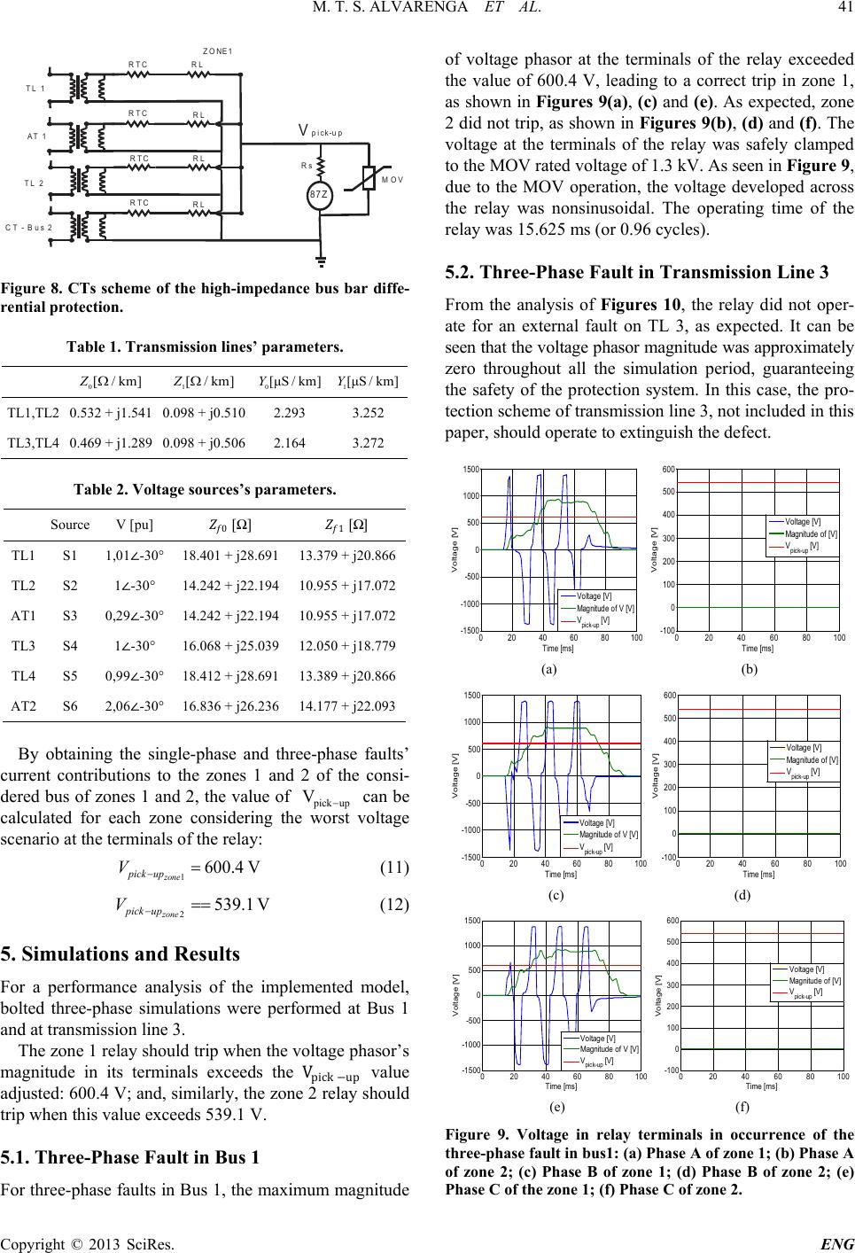

M. T. S. ALVARENGA ET AL.

Figure 8. CTs scheme of the high-impedance bus bar diffe-

rential protection.

Table 1. Transmission lines’ parameters.

[/ km]ZΩ

0[μS/ km]Y

1[μS/ km]Y

TL1,TL2 0.532 + j1.541 0.098 + j0.510 2.293 3.252

TL3,TL4 0.469 + j1.289 0.098 + j0.506 2.164 3.272

Table 2. Voltage sources’s parameters.

Source V [pu]

0 [

Ω

]

1 [

Ω

]

TL1 S1 1,01

∠

-30° 18.401 + j28.691 13.379 + j20.866

TL2 S2 1

∠

-30° 14.242 + j22.194 10.955 + j17.072

AT1 S3 0,29

∠

-30° 14.242 + j22.194 10.955 + j17.072

TL3 S4 1

∠

-30° 16.068 + j25.039 12.050 + j18.779

TL4 S5 0,99

∠

-30° 18.412 + j28.691 13.389 + j20.866

AT2 S6 2,06

∠

-30° 16.836 + j26.236 14.177 + j22.093

By obtaining the single-phase and three-phase faults’

current contributions to the zones 1 and 2 of the consi-

dered bus of zones 1 and 2, the value of

pick up

−

can b e

calculated for each zone considering the worst voltage

scenario at the terminals of the relay:

1600.4 V

zone

pick up

V−=

(11)

2539.1V

zone

pick up

−

(12)

5. Simulations and Results

For a performance analysis of the implemented model,

bolted three-phase simulations were performed at Bus 1

and at transmission line 3.

The zone 1 relay should trip when the voltage phasor’s

magnitude in its terminals exceeds the Vpick −up value

adjusted: 600.4 V; and, similarly, the zone 2 relay should

trip when this value e xc e eds 539.1 V.

5.1. Three-Phase Fault in Bus 1

For three -phase faults in Bus 1, the maximum magnitude

of voltage phasor at the terminals of the relay exceeded

the value of 600.4 V, leading to a correct trip in zone 1,

as shown in Figures 9(a), (c) and (e). As expected, zon e

2 did not trip, as shown in Figures 9(b), (d) and (f). Th e

voltage at the terminals of the relay was safely clamped

to the MOV rated voltage of 1.3 kV. As seen in Figure 9,

due to the MOV operation, the voltage developed across

the relay was nonsinusoidal. The operating time of the

relay was 15.625 ms (o r 0. 96 cycles).

5.2. Three-Phase Fault in Transmission Line 3

From the analysis of Figures 10, the relay did not oper-

ate for an external fault on TL 3, as expected. It can be

seen that the voltage phasor magnitude was approximately

zero throughout all the simulation period, guaranteeing

the safety of the protection system. In this case, the pro-

tection scheme of transmission line 3, not included in this

paper, should operate to extinguish the defect.

(a) (b)

(e) (f)

Figure 9. Voltage in relay terminals in occurrence of the

three-phase fault in bus1: (a) Phase A of zone 1; (b) Phase A

of zone 2; (c) Phase B of zone 1; (d) Phase B of zone 2; (e)

Phase C of the zone 1; (f) Phase C of zone 2.

87Z

Vpick-up

RTC RL

RTC

ZONE1

TL 1

AT 1

CT - Bus 2

TL 2

MOV

020 40 60 80 100

-1500

-1000

-500

500

1000

1500

Time [ms]

Voltage [V]

Voltage [V ]

Ma gnitude of V [V]

pick-up

[V]

020 40 60 80 100

-100

100

200

300

400

500

600

Time [ms]

Voltage [V]

Voltage [V ]

Ma gnitude of [ V ]

pick-up

[V]

020 40 6080 100

-1500

-1000

-500

500

1000

1500

Time [ms]

Voltage [V]

Voltage [V ]

Ma gnitude of V [V]

Vpick- up [V]

020 4060 80100

-100

100

200

300

400

500

600

Time [ms]

Voltage [V]

Voltage [V ]

Ma gnitude of [ V ]

pick-up

[V]

020 40 6080100

-1500

-1000

-500

500

1000

1500

Time [ms]

Voltage [V]

Volta ge [V]

M agni tude of V [V]

pick- up

[V]

020 40 60 80100

-100

100

200

300

400

500

600

Time [ms]

Voltage [V]

Volta ge [V]

M agni tude of [V]

pick- up

[V]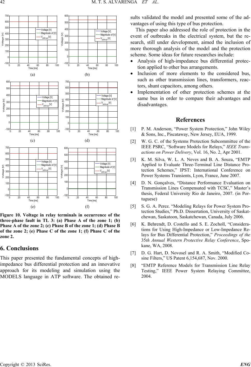

M. T. S. ALVARENGA ET AL.

(a) (b)

(e) (f)

Figure 10. Voltage in relay terminals in occurrence of the

three-phase fault in TL 3: (a) Phase A of the zone 1; (b)

Phase A of the zone 2; (c) Phase B of the zone 1; (d) Phase B

of the zone 2; (e) Phase C of the zone 1; (f) Phase C of the

zone 2.

6. Conclusions

This paper presented the fundamental concepts of high-

impedance bus differential protection and an innovative

approach for its modeling and simulation using the

MODELS language in ATP software. The obtained re-

sults validated the model and presented some of the ad-

vantages of using this type of bus protection.

This paper also addressed the role of protection in the

event of outbreaks in the electrical system, but the re-

search, still under development, aimed the inclusion of

more thorough analysis of the model and the protection

scheme. Some ideas for future researches include:

• Analysis of high-impedance bus differential protec-

tion applied to other bus arrangements.

• Inclusion of more elements to the considered bus,

such as other transmission lines, transformers, reac-

tors, shunt capacitors, among others.

• Implementation of other protection schemes at the

same bus in order to compare their advantages and

disadvantages.

References

[1] P. M. Anderson, “Power System Protection,” John Wiley

& Sons, Inc., Piscataway, New Jersey, EUA, 1999.

[2] W. G. C. of the Systems Protection Subcommittee of the

IEEE PSRC, “Software Models for Relays,” IEEE Trans-

actions on Power Delivery, Vol. 16, No. 2, Apr 2001.

[3] K. M. Silva, W. L. A. Neves and B. A. Souza, “EMTP

Applied to Evaluate Three-Terminal Line Distance Pro-

tection Schemes,” IPST: International Conference on

Power Systems Transients, Lyon, France, June 2007.

[4] D. N. Gonçalves, “Distance Performance Evaluation on

Transmission Lines Compensated with TCSC,” Master’s

thesis, Federal University Rio de Janeiro, 2007. (in Por-

tuguese)

[5] S. G. A. Perez. “Modeling Relays for Power System Pro-

tection Studies,” Ph.D. Dissert ation, University of Saskat-

chewan, Saskatoon, Saskatchewan, Canada, July 2006.

[6] K. Behrendt, D. Costello and S. E. Zocholl, “Considera-

tions for Using High-Impedance or Low-Impedance Re-

lays for Bus Differential Protection,” Proceedings of the

35th Annual Western Protective Relay Conference, Spo-

kane, WA, 2008.

[7] D. G. Hart, D. Novosel and R. A. Smith, “Modified Co-

sine Filters,” US Pate nt 6,154,687, Nov. 2000.

[8] “EMTP Reference Models for Transmission Line Relay

Testing,” IEEE Power System Relaying Committee,

2004.

020 4060 80100

-100

100

200

300

400

500

600

700

Time [ms]

Voltage [V]

Voltage [V ]

Ma gnitude of [ V ]

pick-up

[V]

020 4060 80100

-100

100

200

300

400

500

600

Time [ms]

Voltage [V]

Voltage [V ]

Ma gnitude of [ V ]

pick-up

[V]

020 4060 80 100

-100

100

200

300

400

500

600

Time [ms]

Voltage [V]

Voltage [V ]

Ma gnitude of [ V ]

pick-up

[V]

020 40 60 80 100

-100

100

200

300

400

500

600

700

Time [ms]

Voltage [V]

Voltage [V ]

Ma gnitude of [ V ]

pick-up

[V]

020 40 60 80 100

-100

100

200

300

400

500

600

700

Time [ms]

Voltage [V]

Voltage [V ]

Ma gnitude of [V]

Vpick- up [V]

020 4060 80100

-100

100

200

300

400

500

600

Time [ms]

Voltage [V]

Voltage [V ]

Ma gnitude of [ V ]

pick-up

[V]