A Method for Assessing Customer Harmonic Emission Level Based on the Iterative Algorithm for Least Square Estimation

doi:10.4236/eng.2013.59B002

Engineering, 2013, 5, 6-13

http://dx.doi.org/10.4236/eng.2013.59B002 Published Online September 2013 (http://www.scirp.org/journal/eng)

A Method for Assessing Customer Harmonic Emission

Level Based on th e Iterative Algorithm for

Least Square Estimation*

Runrong Fan, Tianyuan Tan, Hui Chang, Xiaoning Tong, Yunpeng Gao

School of Electrical Engineering, Wuhan University, Wuhan, China

Email: [email protected], [email protected]

Received June 2013

ABSTRACT

With the power system harmonic pollution problems becoming more and more serious, how to distinguish the harmonic

responsibility accurately and solve the grid harmonics simply and effectively has become the main development direc-

tion in harmonic control subjects. This paper, based on linear regression analysis of basic equation and improvement

equation, deduced the least squ ares estimation (LSE) iterative algorithm and obtained the real -time estimates of regres-

sion coefficients, and then calculated the level of the harmonic impedance and emission estimates in real time. This

paper used power system simulation software Matlab/Simulink as analysis tool and analyzed the user side of the har-

monic amplitude and phase fluctuations PCC (point of common coupling) at the harmonic emission level, thus the re-

search has a certain theoretical significance. The development of this algorithm combined with the instrument can be

used in practical engineering.

Keywords: Harmonic Emission Levels; Harmonic Analysis; Least Square Estimation; Iterative Algor ithm

1. Introduction

In the modern power grid system, the traditional power

equipment has gradually been replaced by smart devices

which were based on power electronics and other non-

linear element. Meanwhile, nonlinear loads of the user

side were heavier and heavier. It made the harmonic pol-

lution problems more serious and harmful to the safe

operation of the power system. Besides, the users faced a

great power loss. With the public’s increasing emphasis

on harmonic problems, the user’s reasonable assessment

of harmonic emission levels in public connection point

became an important content of harmonic control [1].

The research of Emission level estimation of harmonic

source was focused on harmonic source qualitative anal-

ysis and quantitative estimates at home and abroad: ac-

tive power direction method [2] was widely used in en-

gineering harmonic source qualitative analysis method.

However, this method is affected deeply by the phase

difference between the harmonic sources. And there is a

big area of uncertainty, so it was not suitable for complex

power systems. Harmonic source in quantitative analysis,

also known as harmonic source emission level assess-

ment, can be divided into intervention type and non-in-

tervention type [3]. Intervention type need to inject into

the system disturbance artificially, which not only in-

creased the cost of harmonic analysis, also limited the

scope of its application. Non-intervention type was dif-

ferent; it could use harmonic source fluctuations of itself

to estimate the harmonic impedance in system without

interfering with its normal operation. This method was

simple to use, easy to the development of equipments. It

has made a great difference in practice [4]. At present,

the main non-invasive methods included fluctuations

method [5,6], the linear regression method [8,9] and the

reference impedance method [7]. Among them, fluctua-

tions method and linear regression method were based on

the condition that system harmonic impedance and

equivalent systems invariant harmonic voltage source

and the load harmonic impedance and equivalent load

harmonic current source change greatly (or vice versa), it

cannot be applied in a steady state harmonic source, and

cannot applied in the condition while the system and user

harmonic source volatility at the same [5-9]. The main

disadvantage of the reference impedance method is that it

needs to get more accurate prior reference impedance [7].

This paper proposed the iterative algorithm for least

square estimation is based on the linear regression analy-

sis of basic equation and the improvement equation. And

*Supported by “the Fundamental Research Funds for the Central Uni-

versities” (Grant No: 207-274592);

Supported by NSFC (Grant No:

51007066)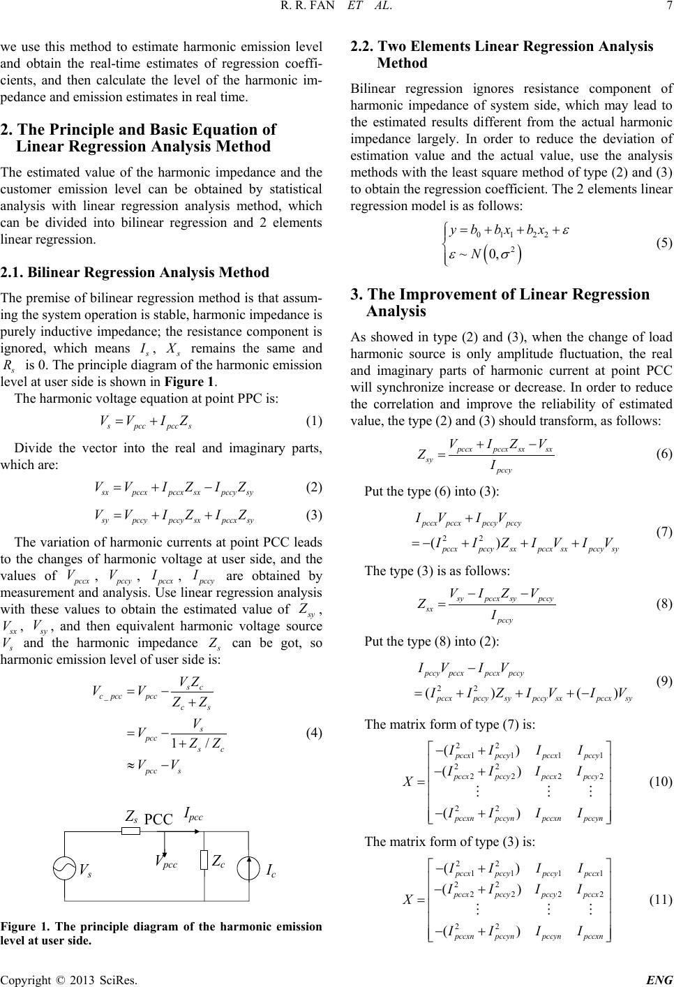

R. R. FAN ET AL.

7

we use this method to estimate harmonic emission level

and obtain the real-time estimates of regression coeffi-

cients, and then calculate the level of the harmonic im-

pedance and emission estimates in real time.

2. The Principle and Basic Equation of

Linear Regression Analysis Method

The estimated value of the harmonic impedance and the

customer emission level can be obtained by statistical

analysis with linear regression analysis method, which

can be divided into bilinear regression and 2 elements

linear regression.

2.1. Bilinear Regression An alysis Method

The premise of bilinear regression method is that assum-

ing the system operation is stable, harmonic impedance is

purely inductive impedance; the resistance component is

ignored, which means

s

I

, s

X

remains the same and

s

R

is 0. The principle diagram of the harmonic emission

level at user side is shown in Figure 1.

The harm onic voltage equatio n at point PPC i s :

spccpcc s

V VIZ= +

(1)

Divide the vector into the real and imaginary parts,

which are:

sxpccxpccx sxpccy sy

V VIZIZ=+−

(2)

sypccypccy sxpccx sy

V VIZIZ=++

(3)

The variation of harmonic currents at point PCC leads

to the changes of harmonic voltage at user side, and the

values of

pccx

V

,

pccy

V

,

pccx

I

,

pccy

I

are obtained by

measurement and analysis. Use linear regression analysis

with these values to obtain the estimated value of

sy

Z

,

sx

V

,

sy

V

, and then equivalent harmonic voltage source

s

V

and the harmonic impedance

s

Z

can be got, so

harmonic emission level of user side is:

_

1/

sc

c pccpcccs

s

pcc sc

pcc s

VZ

VV

ZZ

V

VZZ

VV

=− +

≈−

(4)

V

s

Z

s

PCC I

pcc

V

pcc

Z

c

I

c

Figure 1. The principle diagram of the harmonic emission

level at user side.

2.2. Two Elements Linear Regression Analysis

Method

Bilinear regression ignores resistance component of

harmonic impedance of system side, which may lead to

the estimated results different from the actual harmonic

impedance largely. In order to reduce the deviation of

estimation value and the actual value, use the analysis

methods with the least square method of type (2) and (3)

to obtain the regression coefficient. The 2 elements linear

regression model is as follows:

( )

0112 2

2

~ 0,

y bbxbx

N

ε

εσ

=++ +











(5)

3. The Improvement of Linear Regression

Analysis

As showed in type (2) and (3), when the change of load

harmonic source is only amplitude fluctuation, the real

and imaginary parts of harmonic current at point PCC

will synchronize increase or decrease. In order to reduce

the correlation and improve the reliability of estimated

value, the type (2) and (3) should transform, as follows:

pccxpccx sxsx

sy pccy

V IZV

ZI

+−

=

(6)

Put the type (6) into (3):

22

()

pccx pccxpccy pccy

pccx pccysx pccxsx pccysy

IV IV

IIZIV IV

+

=−+++

(7)

The type (3) is as follows:

sypccx sypccy

sx pccy

VIZ V

ZI

−−

=

(8)

Put the type (8) into (2):

22

( )()

pccy pccxpccx pccy

pccxpccysypccy sxpccxsy

IV IV

IIZ IVI V

−

= +++−

(9)

The matrix form of type (7) is:

22

1111

22

22 22

22

()

pccx pccypccxpccy

pccxn pccynpccxnpccyn

II II

X

II II



−+



−+



=



−+





 

(10)

The matrix form of type (3) is:

22

111 1

22

22 22

22

()

pccx pccypccypccx

pccxn pccynpccynpccxn

II II

X

II II



−+



−+



=



−+





 

(11)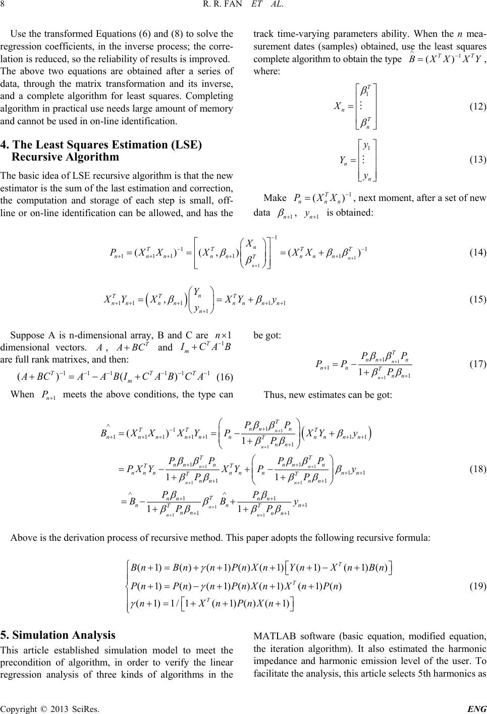

R. R. FAN ET AL.

8

Use the transformed Equations (6) and (8) to solve the

regression coefficients, in the inverse process; the corre-

lation is reduced, so the reliability of results is improved.

The above two equations are obtained after a series of

data, through the matrix transformation and its inverse,

and a complete algorithm for least squares. Completing

algorithm in practical use needs large amount of memory

and cannot be used in on-line identification.

4. The Least Squares Estimation (LSE)

Recursive Algorithm

The basic idea of LSE recursive algorithm is that the new

estimator is the sum of the last estimation and corr ection,

the computation and storage of each step is small, off-

line or on-line identification can be allowed, and has the

track time-varying parameters ability. When the n mea-

surement dates (samples) obtained, use the least squares

complete algorithm to obtain the type

1

()

TT

BXX XY

∧−

=

,

where:

1

T

n

T

n

X

β





=







(12)

1

n

y

Y

y





=







(13)

Make

1

()

T

n nn

P XX

−

=

, next moment, after a set of new

data

1n

β

+

,

1n

y

+

is obtained:

1

11

1 1111

()(, )()

n

T TTT

nnnn nnnn

T

X

PX XXXX

β ββ

β

+

−

−−

+ ++++





=== +











(14)

( )

11 111

1

,

n

TT T

n nnnnnnn

n

Y

X YXXYy

y

ββ

++++ +

+



== +





(15)

Suppose A is n-dimensional array, B and C are

1n×

dimensional vectors.

A

,

T

A BC+

and

1T

m

I CAB

−

+

are full rank matrixes, and then:

111111

()( )

T TT

m

A BCAABICABCA

−− −−−−

+=− +

(16)

When

1n

P

+

meets the above conditions, the type can

be got:

1

11

1n

n

T

nn n

nn Tnn

PP

PP P

ββ

+

=− +

(17)

Thus, new estimates can be got:

( )

1

11

1

11 11111

1

11

1

() 1

11

1

n

nn

n

T

nn n

TT T

nnnnnnnnnn

Tnn

TT

nn nnn n

TT

n nnnnnnn

TT

nn nn

T

nn

Tnn

PP

BXXXYPXYy

P

PP PP

PXYXYPy

PP

BB

P

ββ β

ββ

ββββ β

ββ ββ

ββ

+

++

+

∧+

−

++++++ +

+

++

∧∧

+



==−+



+





= −+−



++



=−+

+

1

11

1

n

nn n

Tnn

y

P

β

ββ

+

++

+

(18)

Above is the derivation process of recursive method. This paper adopts the following recursive formula:

( 1)()(1)()(1)( 1)(1)()

( 1)()(1)()( 1)(1)()

( 1)1/1( 1)()(1)

T

BnBnn PnXnYnXn Bn

PnPnn PnXnXn Pn

nX nPnXn

γ



+=+ +++−+





+=− +++





+= +++





(19)

5. Simulation Analysis

This article established simulation model to meet the

precondition of algorithm, in order to verify the linear

regression analysis of three kinds of algorithms in the

MATLAB software (basic equation, modified equation,

the iteration algorithm). It also estimated the harmonic

impedance and harmonic emission level of the user. To

facilitate the analysis, th is article selects 5th harmonics as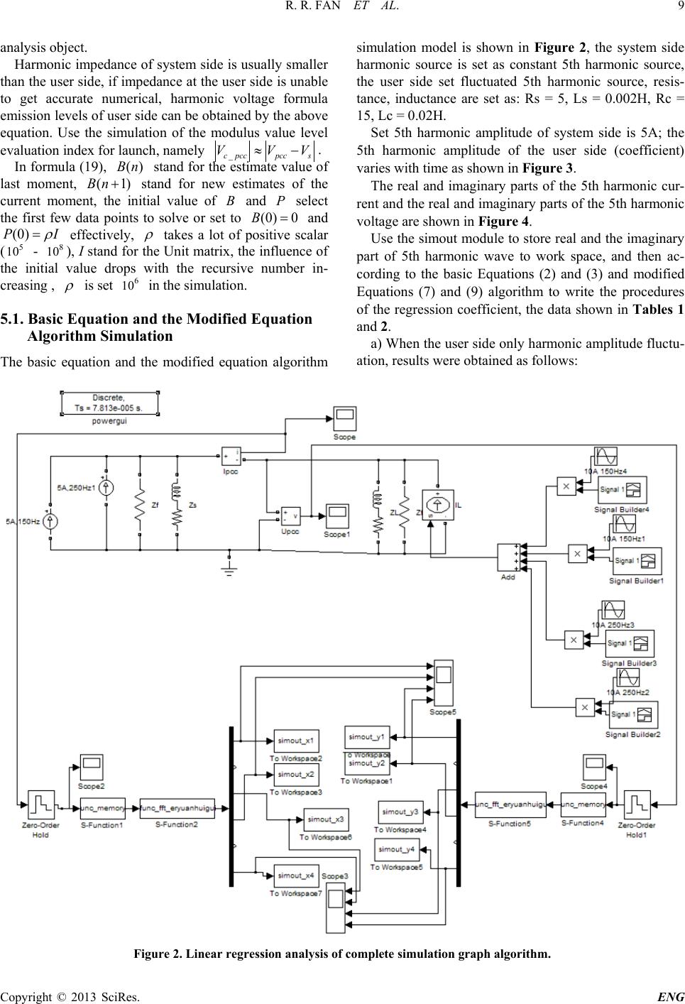

R. R. FAN ET AL.

9

analysis object.

Harmonic impedance of system side is usually smaller

than the user side, if impedance at the user side is unable

to get accurate numerical, harmonic voltage formula

emission levels of user side can be obtained by the above

equation. Use the simulation of the modulus value level

evaluation i ndex for launch, name l y

_cpccpccs

V VV≈−

.

In formula (1 9),

()Bn

stand for the estimate value of

last moment,

( 1)Bn+

stand for new estimates of the

current moment, the initial value of

B

and

P

select

the first few data points to solve or set to

(0) 0B=

and

(0)PI

ρ

=

effectively,

ρ

takes a lot of positive scalar

(5

10 - 8

10 ), I stand for the Unit matrix, the influence of

the initial value drops with the recursive number in-

creasing ,

ρ

is set

6

10

in the simulation.

5.1. Basic Equation and the Modified Equation

Algorithm Simulation

The basic equation and the modified equation algorithm

simulation model is shown in Figure 2, the system side

harmonic source is set as constant 5th harmonic source,

the user side set fluctuated 5th harmonic source, resis-

tance, inductance are set as: Rs = 5, Ls = 0.002H, Rc =

15, Lc = 0.02H.

Set 5th harmonic amplitude of system side is 5A; the

5th harmonic amplitude of the user side (coefficient)

varies with time as shown in Figure 3.

The real and imaginary parts of the 5th harmonic cur-

rent and the real and imaginary parts of the 5th harmonic

voltage are shown in Fig ure 4.

Use the simout module to store real and the imaginary

part of 5th harmonic wave to work space, and then ac-

cording to the basic Equations (2) and (3) and modified

Equations ( 7) and (9) algorithm to write the procedures

of the regression coefficient, the data shown in Tables 1

and 2.

a) When the user side only harmonic amplitude fluctu-

ation, results were obtained as follows:

Figure 2. Linear regression analysis of complete simulation graph algorithm.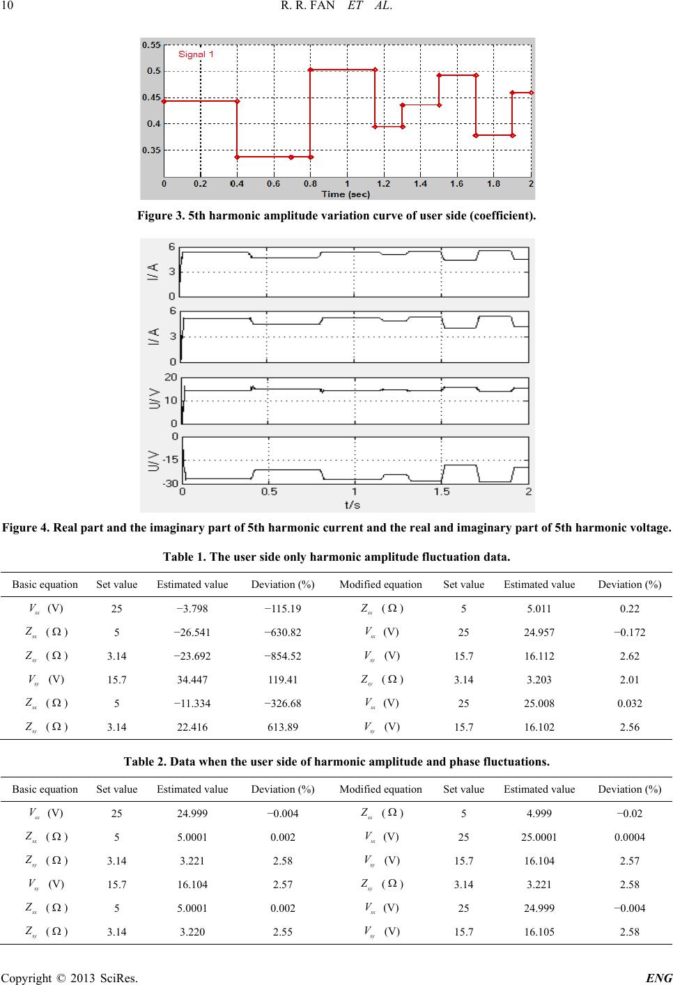

R. R. FAN ET AL.

10

Figure 3. 5th harmonic amplitude variation curve of user side (coefficient).

Figure 4. Real part and the imaginary part of 5th harmonic current and the real and imaginary part of 5th harmonic voltage.

Table 1. The user side only harmonic amplitude fluctuation data.

Basic equation Set value Estimated value Deviation (%) Modified equation Set value Estimated value Deviation (%)

sx

V

(V) 25 −3.798 −115.19

sx

Z

(Ω) 5 5.011 0.22

sx

Z

(Ω) 5 −26.541 −630.82

sx

V

(V) 25 24.957 −0.172

sy

Z

(Ω) 3.14 −23.692 −854.52

sy

V

(V) 15.7 16.112 2.62

sy

V

(V) 15.7 34.447 119.41

sy

Z

(Ω) 3.14 3.203 2.01

sx

Z

(Ω) 5 −11.334 −326.68

sx

V

(V) 25 25.008 0.032

sy

Z

(Ω) 3.14 22.416 613.89

sy

V

(V) 15.7 16.102 2.56

Table 2. Data when the user side of harmonic amplitude and phase fluctuations.

Basic equation Set v alue Estimated value Deviation (%) Modified equation Set value Estimated value Deviation (%)

sx

V

(V) 25 24.999 −0.004

sx

Z

(Ω) 5 4.999 −0.02

sx

Z

(Ω) 5 5.0001 0.002

sx

V

(V) 25 25.0001 0.0004

sy

Z

(Ω) 3.14 3.221 2.58

sy

V

(V) 15.7 16.104 2.57

sy

V

(V) 15.7 16.104 2.57

sy

Z

(Ω) 3.14 3.221 2.58

sx

Z

(Ω) 5 5.0001 0.002

sx

V

(V) 25 24.999 −0.004

sy

Z

(Ω) 3.14 3.220 2.55

sy

V

(V) 15.7 16.105 2.58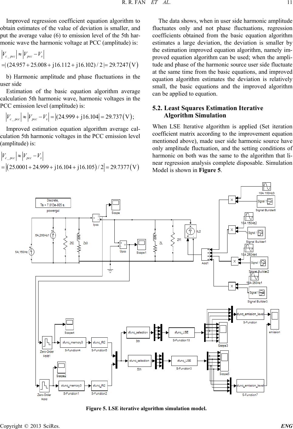

R. R. FAN ET AL.

11

Improved regression coefficient equation algorithm to

obtain estimates of the value of deviation is smaller, and

put the average value (6) to emission level of the 5th har-

monic wave the harmonic voltage at PCC (amplitude) is:

( )

_

| (24.95725.008j16.112j16.102) / 2 |29.7247V

c pccpccs

V VV≈−

=++ +=

b) Harmonic amplitude and phase fluctuations in the

user side

Estimation of the basic equation algorithm average

calculation 5th harmonic wave, harmonic voltages in the

PCC emission level (amplitude) is:

( )

_

(24.999j16.10429.737 V ;

c pccpccs

V VV≈ −=+=

Improved estimation equation algorithm average cal-

culation 5th harmonic voltages in the PCC emission lev el

(amplitude) is:

() ( )

_

25.000124.999 j16.104 j16.105/229.7377V

c pccpccs

V VV≈−

=++ +=

The data shows, when in user side harmonic amplitude

fluctuates only and not phase fluctuations, regression

coefficients obtained from the basic equation algorithm

estimates a large deviation, the deviation is smaller by

the estimation improved equation algorithm, namely im-

proved equation algorithm can be used; when the ampli-

tude and phase of the harmonic source user side fluctuate

at the same time from the basic equations, and improved

equation algorithm estimates the deviation is relatively

small, the basic equations and the improved algorithm

can be applied to equation.

5.2. Least Squares Estimation Iterative

Algorithm Simulation

When LSE Iterative algorithm is applied (Set iteration

coefficient matrix according to the improvement equation

mentioned above), made user side harmonic source have

only amplitude fluctuation, and the setting conditions of

harmonic on both was the same to the algorithm that li-

near regression analysis complete disposable. Simulation

Model is shown in Figure 5.

Figure 5. LSE iterative algorithm simulation model.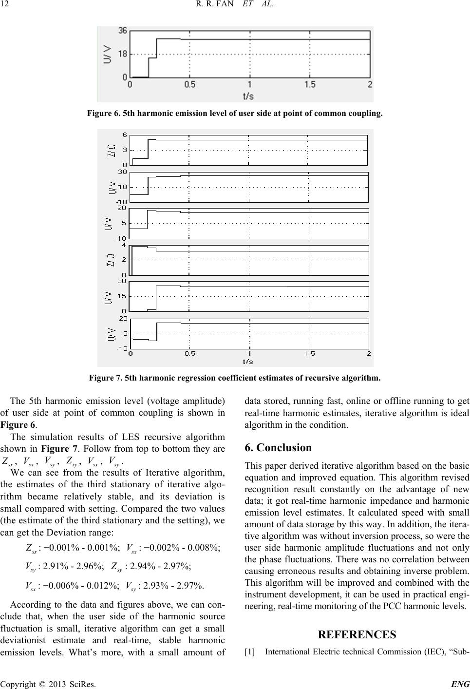

R. R. FAN ET AL.

12

Figure 6. 5th harmonic emission level of user side at point of common coupling.

Figure 7. 5th harmonic regression coefficient estimates of recursive algorithm.

The 5th harmonic emission level (voltage amplitude)

of user side at point of common coupling is shown in

Figure 6.

The simulation results of LES recursive algorithm

shown in Figure 7. Follow from top to bottom they ar e

sx

Z

,

sx

V

,

sy

V

,

sy

Z

,

sx

V

,

sy

V

.

We can see from the results of Iterative algorithm,

the estimates of the third stationary of iterative algo-

rithm became relatively stable, and its deviation is

small compared with setting. Compared the two values

(the estimate of the third stationary and the setting), we

can get the Deviation range:

sx

Z

: −0.001% - 0.001%;

sx

V

: −0.002% - 0.008%;

sy

V

: 2.91% - 2.96%; sy

Z

: 2.94% - 2.97%;

sx

V

: −0.006% - 0.012%;

sy

V

: 2.93% - 2.97%.

According to the data and figures above, we can con-

clude that, when the user side of the harmonic source

fluctuation is small, iterative algorithm can get a small

deviationist estimate and real-time, stable harmonic

emission levels. What’s more, with a small amount of

data stored, running fast, online or offline running to get

real-time harmonic estimates, iterative algorithm is ideal

algorithm in the condition.

6. Conclusion

This paper derived iterative algorithm based on the basic

equation and improved equation. This algorithm revised

recognition result constantly on the advantage of new

data; it got real-time harmonic impedance and harmonic

emission level estimates. It calculated speed with small

amount of data storage by this way. In addition, the itera-

tive algorithm was withou t inversion process, so were the

user side harmonic amplitude fluctuations and not only

the phase fluctuations. There was no correlation between

causing erroneous results and obtaining inverse problem.

This algorithm will be improved and combined with the

instrument development, it can be used in practical engi-

neering, real-time monitoring of t he P CC harmoni c l evels .

REFERENCES

[1] International Electric technical Commission (IEC), “Sub-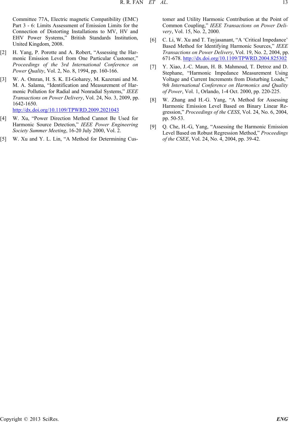

R. R. FAN ET AL.

13

Committee 77A, Electric magnetic Compatibility (EMC)

Part 3 - 6: Limits Assessment of Emission Limits for the

Connection of Distorting Installations to MV, HV and

EHV Power Systems,” British Standards Institution,

United Kingdom, 2008.

[2] H. Yang, P. Porotte and A. Robert, “Assessing the Har-

monic Emission Level from One Particular Customer,”

Proceedings of the 3rd International Conference on

Power Quality, Vol. 2, No. 8, 1994, pp. 160-166.

[3] W. A. Omran, H. S. K. EI-Goharey, M. Kazerani and M.

M. A. Salama, “Identification and Measurement of Har-

monic Pollution for Radial and Nonradial Systems,” IEEE

Transactions on Power Delivery, Vol. 24, No. 3, 2009, pp.

1642-1650.

http://dx.doi.org/10.1109/TPWRD.2009.2021043

[4] W. Xu, “Power Direction Method Cannot Be Used for

Harmonic Source Detection,” IEEE Power Engineering

Society Summer Meeting, 16-20 July 2000, Vol. 2.

[5] W. Xu and Y. L. Lin, “A Method for Determining Cus-

tomer and Utility Harmonic Contribution at the Point of

Common Coupling,” IEEE Transactions on Power Deli-

very, Vol. 15, No. 2, 2000.

[6] C. Li, W. Xu and T. Tayjasanant, “A ‘Critical Impedance’

Based Method for Identifying Harmonic Sources,” IEEE

Transactions on Power Delivery, Vol. 19, No. 2, 2004, pp.

671-678. http://dx.doi.org/10.1109/TPWRD.2004.825302

[7] Y. Xiao, J.-C. Maun, H. B. Mahmoud, T. Detroz and D.

Stephane, “Harmonic Impedance Measurement Using

Voltage and Current Increments from Disturbing Loads,”

9th International Conference on Harmonics and Quality

of Power, Vol. 1, Orlando, 1-4 Oct. 2000, pp. 220-225.

[8] W. Zhang and H.-G. Yang, “A Method for Assessing

Harmonic Emission Level Based on Binary Linear Re-

gression,” Proceedings of the CESS, Vol. 24, No. 6, 2004,

pp. 50-53.

[9] Q. Che, H.-G, Yang, “Assessing the Harmonic Emission

Level Based on Robust Regression Method,” Proceedings

of the CSEE, Vol. 24, No. 4, 2004, pp. 39-42.

Paper Menu >>

Journal Menu >>