RSS Based Bridge Scour Measurement Using Underwater Acoustic Sensor Networks

doi:10.4236/cn.2013.53B2115

Paper Menu >>

Journal Menu >>

Communications and Network, 2013, 5, 641-648

http://dx.doi.org/10.4236/cn.2013.53B2115 Published Online September 2013 (http://www.scirp.org/journal/cn)

RSS Based Bridge Scour Measurement Using Underwater

Acoustic S ensor N etworks

Prabhat Dahal, Dongming Peng, Yaoqing (Lamar) Yang, Hamid Sharif

Department of Computer and Electronics Engineering, University of Nebraska-Lincoln, Lincoln, USA

Email: [email protected]

Received July 2013

ABSTRACT

Bridge Scour is one of the major causes of bridge failures all around the world and there have been significant efforts

for its detection and measurement using different acoustic approaches. In this paper, we propose and investigate an ef-

fective method to utilize Received Signal Strength (RSS) for measuring scour depth where acoustic sensors are dep-

loyed. We also extend a statistical testing to determine the difference in signal levels at the sensor nodes prior to and

after scour formation and subsequently determine the actual depth of scour. Additionally, we make an attempt to eva-

luate underwater distance and depth using signal strength perceived at the receiver which makes it free from the re-

quirement of accurate receiver-sender synchronization in contrast to Time of Flight (ToF) or Time of Arrival (ToA)

techniques. The scour depths are eventually compared for the conditions when the bottom is composed of a single or

multiple layers. The simulation results clearly show that different depths are calculated for the case of multilayered bo t-

tom (0.8 to 3.9 meters for instance) as compared to a constant depth of 2 meters for the case of a single layered bottom.

Keywords: Bridge Scour; Received Signal Strength; Acoustic Wave Propagation; Underwater Acoustic Sensor

Network s

1. Introduction

Bridge scour is considered to be one of the main causes

of bridge failures all over the world. For instance, tenta-

tively 60% of more than 1000 bridge collapses in the

United States in the past 30 years are linked to the scour

of bridge founda tions [1]. The problem of such gravity is

further aggravated by the fact that the annual cost for

scour-related bridge failures only, was estimated to be

around $30 million, according to a study by the Trans-

portation Research Board in 1997 [2].

The process of formation of a bridge scour can be cre-

dited to the erosive action of flowing water. Flowing

water tends to excavate and carry with it sediment mate-

rials from the water bed and from around the bridge col-

umns, piers and abutments. Formation of bridge scour is

a complex and dynamic process that depends on factors

such as the water depth, pier and abutment shape and

width, the velocity of flow, composition and material

properties of the sediments underneath the water body,

and many more. Normally, three different types of scours

are considered-local scour, contraction scour and degra-

dational scour. Local scour is the type that we are dealing

with in this paper, which is the washing away of sedi-

ments from around piers and abutments creating scour

holes.

Several means have been tried for the measurement of

scour depth in the field. Early on, radar and sonar were

employed to successfully measure t he sco ur dep th. R adar

sends out electromagnetic waves to the water bottom,

which then reflects off the bottom interface and reaches

the transmitter. Similarly, sonar is a technique that uses

sound propagation in the same way as a radar does. So-

nar is specifically used for underwater purposes. The time

taken by the radar and sonar waves to travel from trans-

mitter to the receiver after undergoing reflection off the

bottom is used to compute the range and hence the depth.

Despite being successful in measuring scour depth, the

use of radar and sonar is limited by the fact that they are

usually only used to determine the final stage of the se-

diment distribution around the pier and there is no conti-

nuous monitoring. In recent years, techniques employing

Time-Domain Reflectometry (TDR) [3] and Fiber Bragg

Grating (FBG) sensors [4] have emerged to facilitate

real-time monitoring of bridge scour. It is to be noted that

several mechanical systems also exist for the measure-

ment of bridge scour, with one of them being sliding

magnetic collar [5]. However, the major issue with this

system is that it suffers from the problem of jamming and

cannot be reversed for reuse.

Recently, water bottom sensor nodes have been consi-

P. DAHAL ET AL.

642

dered to extend applications beyond underwater environ-

ment monitoring like pollution monitoring, oceanographic

data collection and offshore exploration, and used for

bridge monitoring and tactical surveillance. In order to

achieve this, we need to establish communication be-

tween underwater devices. Underwater Acoustic Sensor

Networks (Underwater-ASN) consist of a variable num-

ber of sensors that are deployed to conduct the task of

collaborative monitoring over a particular area of interest.

However, there are several hindrances when it comes to

the deployment of underwater acoustic sensors. Under-

water acoustic communications are mainly influenced by

path loss, noise, multi-path, Doppler spread and high and

variable propagation delay. All these factors combine to

affect the temporal and spatial variability of the under-

water acoustic channel and make the available bandwidth

of the Underwater Acoustic (UWA) channel limited and

dramatically dependent on both range and frequency. Pro-

vided that underwater acoustic channel has several com-

plexities as such, long-range systems may have a band-

width of only a few KHz, while short-range systems may

have a more than a hundr e d KHz bandwidth.

The rest of the paper is organized as follows: Section

II describes how distances or depths can be estimated by

Received Signal Strength (RSS) method. Section III pro-

vides a detail of the proposed architecture explaining how

the sensors are positioned and the signals are received to

make estimations. Section IV includes the simulation

results that point out the deviation in scour depth from

normal when multilayered bottom is taken into account.

Finally, Section V presents our co nc lusion s.

2. RSS Based Range Estimation

There are different techniques that exist for distance mea-

surement in terrestrial wireless communications such as

Time Difference of Arrival (TDoA), T i me of Arrival (ToA),

Received Signal and Strength Indication (RSSI), and An-

gle of Arrival (AoA), to name a few. TDoA uses two

different transmission-media, e.g. Radio Frequency (RF)

and acoustic wave, to estimate the distance between two

nodes. This estimation is based on different arrival times

due to the difference in propagation speeds through the

same medium [6]. But RF is not quite applicable for un-

derwater usage because of its limited propagation in wa-

ter medium caused by high attenuation [7], and therefore,

TDoA is not used in aquatic environment. In contrast,

AoA method is dependent on a direct line-of-sight (LOS)

path from a transmitter to a receiver. This means that

mul t i -path components of the same signal may appear as

signals arriving from different (unwanted) directions and

can lead to erroneous results in AoA measurements [8].

ToA is extensively used for range measurement in short-

range Underwater Acoustic Sensor Networks (UASNs)

[9,10]. As its name refers, it utilizes the time taken by an

acoustic wave to travel from the transmitter to the re-

ceiver [8]. The time taken for travel is used to calculate

the distance according to the underwater sound velocity.

It is worth mentioning that for accurate results using ToA,

the sender and receiver must be accurately synchronized.

For this work, we attempt to make use of a new dis-

tance measurement technique (here, depth) based on Re-

ceived Signal Strength (RSS) for short range underwater

acoustic communications. Unlike ToA, in RSS, wireless

devices use the received signal power to measure the

distance between the sender and the receiver. Seen this

way, synchronization is not a problem as in ToA, but

simplifying the distance/transmission-loss relationship

can be quite complex. The work in [11] shows that the

function to express distance in terms of transmission loss

required by RSS for distance calculation uses the Lam-

bert W function. The distance function is derived after

sufficient iteration functions. The authors claim that a

very accurate calculation of distance can be made in less

than four iterations. We utilize the RSS based range es-

timation approach as proposed by [11] for our research.

Sound loss in water is classified as spreading loss and

attenuation loss. Spr eading loss includes spherical 1) and

cylindrical 2) losses, which is caused by the expansion of

an acoustic wave as it propagates through a medium, and

attenuation includes absorption, scattering and diffrac tion

[12]. Accurate values for attenuation can be measured by

considering the effects of transmission medium (salinity,

pressure, temperature and many others) and environment

parameters like air bubbles within water volume, absorp-

tion by the sediments, reflection off the surfaces and

scattering. Here, only transmission medium parameters

are considered for the ease of calculation. Transmission

losses can be mathematically expressed as

20log( )TLsph Dist=

(1)

10log( )TLcyl Dist=

(2)

where the first equation gives an expression for the trans-

mission loss with respect to spherical propagation of the

wave and the second equation is that with respect to cy-

lindrical propagation. So the general expression for trans-

mission loss in sea water [12] is given by

10TLtotalTLsph TLcylDist

−

= ++

( 3)

where α is the absorption coefficient in sea water as ex-

pressed in (4), given by the Thorp’s absorption coeffi-

cient [13], which depends only on frequency f below 50

kHz,

0.1 40

1.0936

1 4100



= +





(4)

Here, the factor 1.0936 is used to change the unit of

the coefficient from dB/kyd to dB/km. The authors in [11]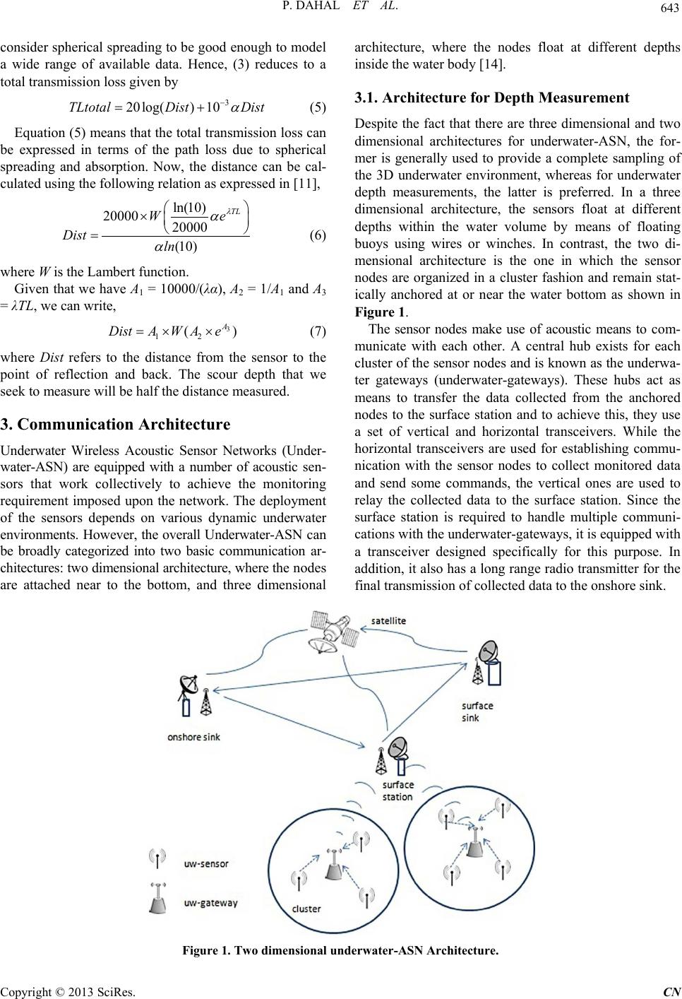

P. DAHAL ET AL.

643

consider spherical spreading to be good enough to model

a wide range of available data. Hence, (3) reduces to a

total transmission loss given by

20log() 10TLtotalDist Dist

−

= +

(5)

Equation (5) means that the total transmission loss can

be expressed in terms of the path loss due to spherical

spreading and absorption. Now, the distance can be cal-

culated using the following rela t ion as expre s s e d in [11],

ln(10)

20000 20000

(10)

Dist ln



×



(6 )

where W is the Lambert function.

Given that we have A1 = 10000/(λα), A2 = 1/A1 and A3

= λTL, we can wri t e ,

( )

DistAW Ae=××

(7 )

where Dist refers to the distance from the sensor to the

point of reflection and back. The scour depth that we

seek to measure will be half the distance measured.

3. Communication Architecture

Underwater Wireless Acoustic Sensor Networks (Under-

water-ASN) are equipped with a number of acoustic sen-

sors that work collectively to achieve the monitoring

requirement imposed upon the network. The deployment

of the sensors depends on various dynamic underwater

environments. However, the overall Un derwater-ASN can

be broadly categorized into two basic communication ar-

chitectures: tw o di mensional arch itectur e, wher e the nodes

are attached near to the bottom, and three dimensional

architecture, where the nodes float at different depths

inside t he wa ter body [14].

3.1. Architecture for Depth Measurement

Despite the fact that there are three dimensional and two

dimensional architectures for underwater-ASN, the for-

mer is generally used to provide a complete sampling of

the 3D underwater environment, whereas for underwater

depth measurements, the latter is preferred. In a three

dimensional architecture, the sensors float at different

depths within the water volume by means of floating

buoys using wires or winches. In contrast, the two di-

mensional architecture is the one in which the sensor

nodes are organized in a cluster fashion and remain stat-

ically anchored at or near the water bottom as shown in

Figure 1.

The sensor nodes make use of acoustic means to com-

municate with each other. A central hub exists for each

cluster of the sensor nodes and is known as the underwa-

ter gateways (underwater-gateways). These hubs act as

means to transfer the data collected from the anchored

nodes to the surface station and to achieve this, they use

a set of vertical and horizontal transceivers. While the

horizontal transceivers are used for establishing commu-

nication with the sensor nodes to collect monitored data

and send some commands, the vertical ones are used to

relay the collected data to the surface station. Since the

surface station is required to handle multiple communi-

cations with the underwater-gateways, it is equipped with

a transceiver designed specifically for this purpose. In

addition, it also has a long range radio transmitter for the

final transmission of collected data to the onshore sink.

Figu re 1. Two dimensional unde rw ate r -ASN Architecture.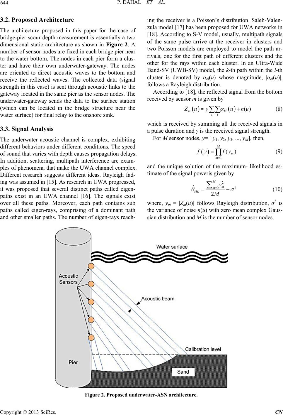

P. DAHAL ET AL.

644

3.2. Proposed Architecture

The architecture proposed in this paper for the case of

bridge-pier scour depth measurement is essentially a two

dimensional static architecture as shown in Figure 2. A

number of sensor nodes are fixed in each bridge pier near

to the water bottom. The nodes in each pier form a clus-

ter and have their own underwater-gateway. The nodes

are oriented to direct acoustic waves to the bottom and

receive the reflected waves. The collected data (signal

strength in this case) is sent through acoustic links to the

gateway located in the same pier as the sensor nodes. The

underwater-gateway sends the data to the surface station

(which can be located in the bridge structure near the

water surface) for final relay to the onshore sink.

3.3. Signal Analysis

The underwater acoustic channel is complex, exhibiting

different behaviors under different conditions. The speed

of sound that varies with dep th cau ses propaga tion dela ys.

In addition, scattering, multipath interference are exam-

ples of phenomena that make the UWA channel complex.

Different research suggests different ideas. Rayleigh fad-

ing was assumed in [15]. As research in UWA progressed,

it was proposed that several distinct paths called eigen-

paths exist in an UWA channel [16]. The signals exist

over all these paths. Moreover, each path contains sub

paths called eigen-rays, comprising of a dominant path

and other smaller paths. The number of eigen-rays reach-

ing the receiver is a Poisson’s distribution. Saleh-Valen-

zula model [17] has been proposed for UWA networks in

[18]. According to S-V model, usually, multipath signals

of the same pulse arrive at the receiver in clusters and

two Poisson models are employed to model the path ar-

rivals, one for the first path of different clusters and the

other for the rays within each cluster. In an Ultra-Wide

Band-SV (UWB-SV) model, the k-th path within the l-th

cluster is denoted by αkl(u) whose magnitude, |αkl(u)|,

follows a Rayleigh distribution.

According to [18], the reflected signal from the bottom

received by senso r m is give n by

( )( )

()

m kl

Z uunu

γα

≈+

∑∑

(8 )

which is received by summing all the received signals in

a pulse duration an d γ is the received signal strength.

For M sensor nodes, y= [ y1, y2, y3, ..., yM], then,

( )

()

fy fy

∏

(9)

and the unique solution of the maximum- likelihood es-

timate of the signal poweris g iven by

ˆ2

θσ

= −

∑

(10)

where, ym = |Zm(u)| follows Rayleigh distribution, σ2 is

the variance of noise n(u) with zero mean complex Gaus-

sian distribution and M is the number of sensor nodes.

Figure 2. Proposed underwater-ASN architecture.

P. DAHAL ET AL.

645

Let us define the estimates of received signal power (θ

= γ2/2) before and after scour formation as

( )( )

11 11

ˆˆ and

ML mML m

θθ

(11)

The estimates are gamma distributed (parameter k and

θ). For sufficiently large number of sensor nodes, the

estimates tend to normal distribution with mean, µ = kθ

and variance = kθ2. Then,

212

ˆ2

θσ

= −

∑

(12)

and

222

θσ

= −

∑

(13)

Given that a scour has been formed, the signal incident

at the bottom now has to undergo an additional path

through water and be reflected off the bottom comprising

of a dense layer of water and a solid half space. It is ob-

vious that the signal reaching the sensor in this case

weakens in strength, owing to the additional transmission

loss and the reflection loss. We seek to calculate the dif-

ference in the estimate at the receiver and difference in

mean of the two estimates is employed for this. In order

to take into account, the effect of the entire distribution

of the estimates, a 95% Confidence Interval (C.I.) is

created that will provide us with a range [a, b], as given

in (15) and (16) between which the difference of mean of

the estimates is likely to exist. We have proven this

through the simulations that the higher the number of

sensors, the more accurate the confidence interval is. For

a 95% significance level (two tailed), the C.I. is given by,

( )

1 212

. .1.96CI

θθ

µµ σ

−

= ±−

(14 )

such that,

( )

1 212

1.96a

θθ

µµ σ

−

=−−

(15)

and

( )

1 212

1.96b

θθ

µµ σ

−

=−+

(1 6)

where a and b are the lower and upper limits of the con-

fidence interval respec tively and 1.96 is the z-value from

the z-table correspo nding to the 95% significance level.

If a and b are both positive in C.I. = [a, b], we are 95%

confident that there has been a decrement in received

signal power. Assuming similar conditions of water and

the environment, the signal has probably travelled addi-

tional path (depth) and there could be a probable scour

forma tion which can be checked for.

The difference in signal power (γ2/2) thus estimated is

due to the additional Transmission Loss and Reflection

Loss (RL). From Figure 3(a), for the condition prior to

scour formati on, we have,

1 011SLSLTL RL= −−

(17)

where SL1 = 20log (

) is the received signal level at the

sensors.

Similarly, after the scour has been formed, as shown in

Figure 3(c), we have the expression for received signal

level at the sensors as,

2 0112 2SLSLTLRL TLRL=−−− −

(18)

where SL2 = 20 log (

) is the received signal level, TL2

is the transmission loss in water with depth d0 and RL2 is

the reflection loss from the layered bottom, with the

depth of se di ment lay e r be i ng d1.

From (17) and (18), we have,

20log2 2 1RL TLRL



= +−





(19)

where RL2 is the reflection loss from the layered bottom

expressed as RL2 = −20log (Rb).

Provided that we make an estimate of γ1 and γ2, we can

calculate RL1, TL2 for a particular depth d1 and this

would lead us to estimate the depth d0 using (7). The total

depth would then be D = d0 + d1. Despite the fact that d1

is the depth of the sediment layer, it should be noted that

this layer is unconsolidated, which is considered liquid

and would n ot provide s upport require d f o r the pier.

In contrast, when the bottom after scour formation is

considered to be a single layered half space, (19) be-

comes

20log 2TL







(20)

with TL2 being accountable for the entire depth D = d0

and d1 = 0.

Figure 3. Reflection and Transmission Losses when (a) no

scour has been formed (b) the bottom is a single layer half-

space and (c) the bottom is composed of unconsolidated

sediment layer over solid half-space.

P. DAHAL ET AL.

646

4. Simulation Results

The simulation results presented in this section are based

on assumed values as given in Table 1 and were imple-

mented in MATLAB on a Intel(R) Core(TM)2Duo 2.00

GHz processor. The frequency of acoustic wave chosen

is 10 KHz which gives a Thorp’s absorption coefficient,

α, equal to 1.1498.

For a significance level of 95%, we have the Confi-

dence Interval (C.I.) as

1 212

. .()1.96CI

θθ

µµ σ

−

=−±

(21 )

where, the z-value 1.96 corresponds to 95% significance

level from the z-table.

Different values of received signal strengths at the sen-

sor nodes are assumed for two different conditions- the

initial one, where the acoustic signals reflect off the solid

half layered bottom, which is taken as a reference; and

the second one, where a scour has been formed and the

bottom has shifted to a certain depth from the reference

level. For the second case, as per our assumption, the

bottom consists of a dense liquid layer atop a solid half

layered bottom, thereby causing the reflected signals

reaching the sensors to be of lesser strength than in the

initial condition.

The graphs in Figure 4 present different instances of

calculated C.I. that indicate that we are 95% confident of

the difference in signal powers between the initial and

the latter condition being in between the lower limit (the

bar on the left) and the upper limit (the bar on the right),

for the case of 50 sensor nodes. The line between the

upper limit and the lower limit in each pair of bars indi-

cate the actual difference in signal levels.

Talbe 1. Assumed Data For Water Bottom Layers.

Layer Thickness cp ( m/s)a cs (m/s)b ρ (g/cm3)

1 1 1700 0 1.8

2 ∞ 4700 1900 2.5

a Compre s si on wave velocity; bShear wave velocity.

Figure 4. Confidence Interval for difference in signal stren-

gth at the receiver (M = 50).

Figure 5 presents similar graphs for the cases of the

number of nodes being 5 and 80 respectively. It can clear-

ly be seen that, as the number nodes increases, the 95%

C.I. of the estimate of difference in signal powers nar-

rows and gets closer to the actual value. The result is the

opposite when the number of sensor nodes is decreased.

This shows that, for our C.I. to be a more accurate repre-

sentation of difference in signal powers, a greater number

of sensor nodes is preferred.

The second section of the simulation, as shown in Fig-

ure 6, comprises of the part where the effect of layered

bottom is compared to non-layered bottom with respect

to scour-depth measurement. For different data, as given

in Table 1, scour depths are measured for the condition

when the bottom is composed of a single layer, and the

condition when the bottom is composed of two layers (a

sediment layer of a certain thickness d1, treated as liquid

and a solid bottom). The graphs present the results for the

signal powers in case 1 of Figure 5, for the case of 80

sensor nodes.

Figure 6 expresses that the total scour depth, for the

same received signal strength, depends on the thickness

of the sediment layer. The bars represent the total depth

(including the additional water depth, d0, and the sedi-

ment layer depth, d1). For each depth, different thickness

Figure 5. Confidence Interval for difference in signal

strength at the receiver (M = 5, M = 80).

Figure 6. Comparison of scour depth with and without

layered bottom. Bars for the layered bottom show the vari-

ation in total depth with the depth of the sediment layer.

P. DAHAL ET AL.

647

of the sediment layer is considered and the water depth is

calculated to account for the total loss in signal strength

as compared to the reference level. As the sediment layer

depth increases (shown by the lower portion of the bars),

the corresponding water layer depth also increases, thus

increasing the total scour depth. For instance, for a 24.63

dB signal loss measured at the receiver (with respect to

the condition when no scour was formed), an assumption

of 0.5 meters sediment layer thickness leads to a total

scour depth of approximately 0.8 meters. Likewise, for

the same signal loss measured, assuming a sediment layer

depth of 2 meters gives a total scour depth of around 1.8

meters.

However, the scour depth without considering the

layered approach (when the bottom is a single layered

half space), as shown by the straight line in Figure 6, is

constant and seems to deviate from the depths calculated

for a layered bottom. This shows that the single layered

approach, which is inconsistent with the real underwater

scenario as pointed out in literature, gives misleading

values for scour depth and the effect of sediment layer

thickness on scour depth cannot be neglected. The for-

mation of dense sediment layer above solid water bottom

results in different val ue s of scour depth.

5. Conclusion

Scour holes that ten d to make bridge foundatio ns weaker

to collapses sh ould be accurately measured. W e have suc-

cessfully shown the RSS for acoustic sensor networks.

Unlike ToF or ToA methods for range measurement in

underwater environment, in this paper we provided RSS

approach to measuring bridge scour depth. Simulations

show that the estimation of scour depth tends to approach

the real depth as the number of acoustic sensors em-

ployed is increased. Also, since in real underwater condi-

tions, erosion of sediments leads to the formation of a

dense water layer over the water bottom due to the dis-

solved sediments, an effort is made to compare the effect

of layered nature of water bottom on scour depth to that

of non-layered approach- the layered approach giving

more accurate values for scour depth. For instance, as

seen in the simulations, a sediment layer depth of 1.5

meters results in a total scour depth of 2.8 meters and this

value increases with the thickness of the sediment layer.

In contrast, when the sing le layered bottom is considered,

the resultant scour depth is about 2 meters. However,

since a single layered bottom assumption is fairly unrea-

listic, the result obtained could be misleading.

6. Acknowledgments

This work was sponsored in part by an Interdisciplinary

Research Grant of the University of Nebraska-Lincoln.

REFERENCES

[1] A. M. Shirhole and R. C. Holt, “Planning for a Compre-

hensive Bridge Safety Program,” Transportation Research

Record No. 1290, Transportation Research Board, Na-

tional Research Council, Washington, D.C., 1991.

[2] P. F. Lagasse, E. V. Richardson, J. D. Schall and G. R.

Price, “Instrumentation for Measuring Scour at Bridge

Piers and Abutments,” National Cooperative Highway

Research Program (NCHRP) Paper No. 396, Transporta-

tion Research Board, National Research Council, Wash-

ington, D.C., 1997.

[3] N. E. Yankielun and L. Zabilansky, “Laboratory Investi-

gation of Time-Domain Reflectometry System for Moni-

toring Bridge Scour,” Journal of Hydraulic Engineering,

Vol. 125, No. 12, 1999, pp. 1279-1284.

http://dx.doi.org/10.1061/(ASCE)0733-9429(1999)125:12

(1279)

[4] Y. B. Lin, J.-C. Chen, K.-C. Chang, J.-C. Chern and J.-S.

Lai, “Real Time Monitoring of Bridge Scour Using Fiber

Bragg Grating Sensors,” Smart Materials and Structures,

Vol. 14, No. 4, 2005, pp. 664-670.

http://dx.doi.org/10.1088/0964-1726/14/4/025

[5] J. -Y. L u, J. -H. Hong, C. -C. Su, C. -Y. Wang and J. -S.

Lai, “Field Measurements and Simulation of Bridge

Scour Depth Variation During Floods,” Journal of Hy-

draulic Engineering, Vol. 134, No. 6, 2008, pp. 810-821.

http://dx.doi.org/10.1061/(ASCE)0733-9429(2008)134:6(

810)

[6] N. B. Priyantha, A. Chakraborty and H. Balakrishnan,

“Cricket Location Support System,” Proceedings of the

Annual International Conference on Mobile Computing

and Networking, MOBICOM, 2000, pp. 32-43.

[7] J. Heidemann, W. Ye, J. Wills, A. Syed and Y. Li, “Re-

search Challenges and Applications for Underwater Sen-

sor Networking,” IEEE Wireless Communications and

Networking Conference, WCNC, Vol. 1, 2006, pp. 228-

235.

[8] G. Mao, B. Fidan and B. D. Anderson, “Wireless Sensor

Network Localization Techniques,” Computer Networks,

Vol. 51, No. 10, 2007, pp. 2529-2553.

http://dx.doi.org/10.1016/j.comnet.2006.11.018

[9] M. Erol, L. Vieira, A. Caruso, F. Paparella, M. Gerla and

S. Oktug, “Multi Stage Underwater Sensor Localization

Using Mobile Beacons,” Second International Confe-

rence on Sensor Technologies and Applications, 2008.

SENSORCOMM ‘08, 2008, pp. 710-714.

[10] E. Kim, S. Woo, C. Kim and K. Kim, “Lamsm: Localiza-

tion Algorithm with Merging Segmented Maps for Un-

derwater Sensor Networks,” Lecture Notes in Computer

Science (including subseries Lecture Notes in Artificial

Intelligence and Lecture Notes in Bioinformatics), Vol.

4809 NCS, 2007, pp. 445-454.

[11] M. Hosseini, H. Chizari, C. K. Soon and R. Budioarto,

“RSS-Based Distance Measurement in Underwater Acou-

stic Sensor Networks: An Application of the Lambert W

Function,” Proceedings of the 4th International Confe-

rence on Signal Processing and Communication Systems,

ICSPS, Gold Coast, 2010, pp. 1-4.

[12] P. Etter, “Underwater Acoustic Modeling and Simulation,”

P. DAHAL ET AL.

648

3rd Edition, Spon Press, 2003.

http://dx.doi.org/10.4324/9780203417652

[13] W. H. Thorp, “Analytic Description of the Low-Fre-

quency Attenuation Coefﬁcient, ” Acoustical Society of

America Journal, Vol. 42, 1967, p. 270.

http://dx.doi.org/10.1121/1.1910566

[14] I. F. Akyildiz, D. Pompili, T. Melodia, “Challenges for

Efficient Communication in Underwater Acoustic Sensor

Networks,” ACM SIGBED Review-Special Issue on Em-

bedded Sensor Networks, ACM, NY, 2004, pp. 3-8.

[15] J. A. Catipovic, A. B. Baggeroer, K. Von Der Heydt and

D. Koelsch, “Design and Performance Analysis of a Dig-

ital Telemetry System for Short Range Underwater Chan-

nel,” IEEE Journal of Oceanic Engineering, Vol. OE-9,

No. 4, 1984, pp. 242-252.

http://dx.doi.org/10.1109/JOE.1984.1145632

[16] X. Geng and A. Zielinski, “An Eigenpath Underwater

Acoustic Communication Channel Model,” OCEANS ‘95.

MTS/IEEE, Challenges of Our Changing Global Envi-

ronment, Conference Proceedings, Vol. 2, 1995, pp.

1189-1196.

[17] A. A. Saleh and R. A. Valenzuela, “A Statistical Model

for Indoor Multipath Propagation,” IEEE Journal on Se-

lected Areas in Communications, Vol. 5, No. 2, 1987, pp.

128-137.

[18] Q. Liang and X. Cheng, “Underwater Acoustic Sensor

Networks: Target Size Detection and Performance Anal-

ysis,” Proceedings of IEEE International Conference on

Communications, Beijing, May 2008, pp. 3151-3155.