

Paper Menu >>
Journal Menu >>
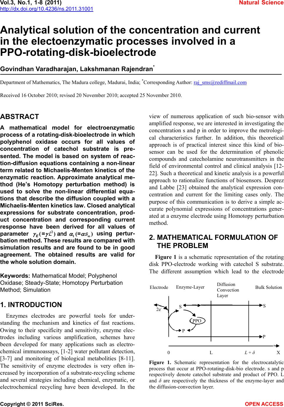 Vol.3, No.1, 1-8 (2011) Natural Science http://dx.doi.org/10.4236/ns.2011.31001 Copyright © 2011 SciRes. OPEN ACCESS Analytical solution of the concentration and current in the electoenzymatic processes involved in a PPO-rotating-disk-bioelectrode Govindhan Varadharajan, Lakshmanan Rajendran* Department of Mathematics, The Madura college, Madurai, India; *Corresponding Author: [email protected] Received 16 October 2010; revised 20 November 2010; accepted 25 November 2010. ABSTRACT A mathematical model for electroenzymatic process of a rotating-disk-bioelectrode in which polyphenol oxidase occurs for all values of concentration of catechol substrate is pre- sented. The model is based on system of reac- tion-diffusion equations containing a non-linear term related to Michaelis-Menten kinetics of the enzymatic reaction. Approximate analytical me- thod (He’s Homotopy perturbation method) is used to solve the non-linear differential equa- tions that describe the diffusion coupled with a Michaelis-Menten kinetics law. Closed analytical expressions for substrate concentration, prod- uct concentration and corresponding current response have been derived for all values of parameter 2 1 ()( )== E and Ls using pertur- bation method. These results are compared with simulation results and are found to be in good agreement. The obtained results are valid for the whole solution domain. Keywords: Mathematical Model; Polyphenol Oxidase; Steady-State; Homotopy Perturbation Method; Simulation 1. INTRODUCTION Enzymes electrodes are powerful tools for under- standing the mechanism and kinetics of fast reactions. Owing to their specificity and sensitivity, enzyme elec- trodes including various amplification, schemes have been developed for many applications such as electro- chemical immunoassays, [1-2] water pollutant detection, [3-7] and monitoring of biological metabolities [8-11]. The sensitivity of enzyme electrodes is very often in- creased by incorporation of a substrate-recycling scheme and several strategies including chemical, enzymatic, or electrochemical recycling have been developed. In the view of numerous application of such bio-sensor with amplified response, we are interested in investigating the concentration s and p in order to improve the metrologi- cal characteristics further. In addition, this theoretical approach is of practical interest since this kind of bio- sensor can be used for the determination of phenolic compounds and catecholamine neurotransmitters in the field of environmental control and clinical analysis [12- 22]. Such a theoretical and kinetic analysis is a powerful approach to rationalize functions of biosensors. Desprez and Labbe [23] obtained the analytical expression con- centration and current for the limiting cases only. The purpose of this communication is to derive a simple ac- curate polynomial expressions of concentrations gener- ated at a enzyme electrode using Homotopy perturbation method. 2. MATHEMATICAL FORMULATION OF THE PROBLEM Figure 1 is a schematic representation of the rotating disk PPO-electrode working with catechol S substrate. The different assumption which lead to the electrode Electrode Enzyme-Layer Diffusion Convection Layer Bulk Solution SS P P PPO 2e - 0L L + δ X Figure 1. Schematic representation for the electrocatalytic process that occur at PPO-rotating-disk-bio electrode. s and p respectively denote catechol substrate and product of PPO. L and δ are respectively the thickness of the enzyme-layer and the diffusion-convection layer. 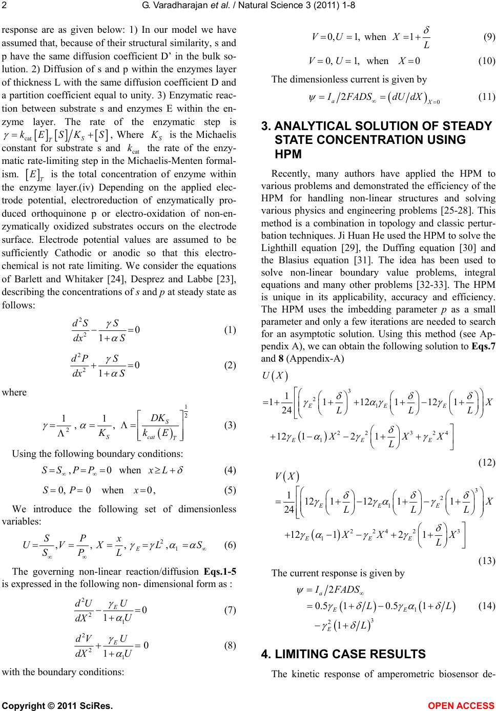 G. Varadharajan et al. / Natural Science 3 (2011) 1-8 Copyright © 2011 SciRes. OPEN ACCESS 2 response are as given below: 1) In our model we have assumed that, because of their structural similarity, s and p have the same diffusion coefficient D’ in the bulk so- lution. 2) Diffusion of s and p within the enzymes layer of thickness L with the same diffusion coefficient D and a partition coefficient equal to unity. 3) Enzymatic reac- tion between substrate s and enzymes E within the en- zyme layer. The rate of the enzymatic step is cat S T kESK S , Where S K is the Michaelis constant for substrate s and cat k the rate of the enzy- matic rate-limiting step in the Michaelis-Menten formal- ism. T E is the total concentration of enzyme within the enzyme layer.(iv) Depending on the applied elec- trode potential, electroreduction of enzymatically pro- duced orthoquinone p or electro-oxidation of non-en- zymatically oxidized substrates occurs on the electrode surface. Electrode potential values are assumed to be sufficiently Cathodic or anodic so that this electro- chemical is not rate limiting. We consider the equations of Barlett and Whitaker [24], Desprez and Labbe [23], describing the concentrations of s and p at steady state as follows: 2 20 1 dS S S dx (1) 2 20 1 dP S S dx (2) where 1 2 2 11 ,, S Scat T DK KkE (3) Using the following boundary conditions: ,0 when SS PPxL (4) 0,0 when 0,SP x (5) We introduce the following set of dimensionless variables: 2 1 ,,, , E SPx UV XLS SP L (6) The governing non-linear reaction/diffusion Eqs.1-5 is expressed in the following non- dimensional form as : 2 2 1 0 1 EU dU U dX (7) 2 2 1 0 1 EU dV U dX (8) with the boundary conditions: 0,1, when 1VUX L (9) 0,1, when 0VU X (10) The dimensionless current is given by 0 2 aX IFADS dUdX (11) 3. ANALYTICAL SOLUTION OF STEADY STATE CONCENTRATION USING HPM Recently, many authors have applied the HPM to various problems and demonstrated the efficiency of the HPM for handling non-linear structures and solving various physics and engineering problems [25-28]. This method is a combination in topology and classic pertur- bation techniques. Ji Huan He used the HPM to solve the Lighthill equation [29], the Duffing equation [30] and the Blasius equation [31]. The idea has been used to solve non-linear boundary value problems, integral equations and many other problems [32-33]. The HPM is unique in its applicability, accuracy and efficiency. The HPM uses the imbedding parameter p as a small parameter and only a few iterations are needed to search for an asymptotic solution. Using this method (see Ap- pendix A), we can obtain the following solution to Eqs.7 and 8 (Appendix-A) 3 2 1 22 324 1 1 11121121 24 12121 EEE EEE UX X LLL XXX L (12) 3 2 1 224 23 1 112 11211 24 12121 EEE EEE VX X LLL XX X L (13) The current response is given by 1 3 2 2 0.510.51 1 a EE E IFADS LL L (14) 4. LIMITING CASE RESULTS The kinetic response of amperometric biosensor de- 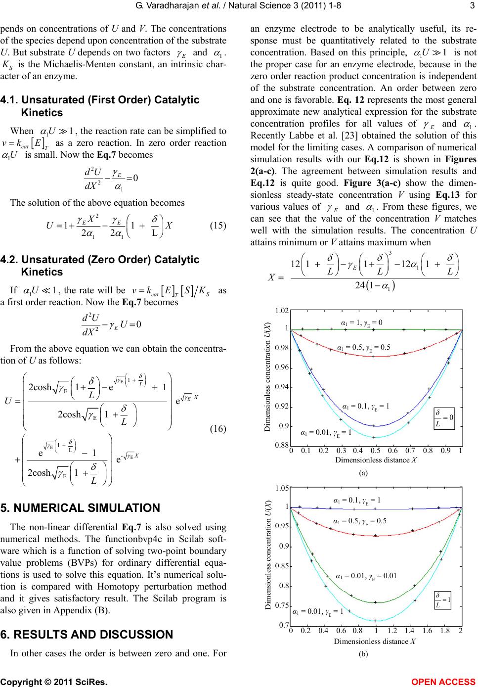 G. Varadharajan et al. / Natural Science 3 (2011) 1-8 Copyright © 2011 SciRes. OPEN ACCESS 33 pends on concentrations of U and V. The concentrations of the species depend upon concentration of the substrate U. But substrate U depends on two factors E and 1 . S K is the Michaelis-Menten constant, an intrinsic char- acter of an enzyme. 4.1. Unsaturated (First Order) Catalytic Kinetics When 11U , the reaction rate can be simplified to cat T vk E as a zero reaction. In zero order reaction 1 U is small. Now the Eq.7 becomes 2 2 1 0 E dU dX The solution of the above equation becomes 2 11 11 22 L EE X UX (15) 4.2. Unsaturated (Zero Order) Catalytic Kinetics If 11U , the rate will be cat S T vk E SK as a first order reaction. Now the Eq.7 becomes 2 20 E dU U dX From the above equation we can obtain the concentra- tion of U as follows: E E E 1 E E 1 L- E 2cosh1e 1 e 2cosh1 e 1 e 2cosh1 E L X X L U L L (16) 5. NUMERICAL SIMULATION The non-linear differential Eq.7 is also solved using numerical methods. The functionbvp4c in Scilab soft- ware which is a function of solving two-point boundary value problems (BVPs) for ordinary differential equa- tions is used to solve this equation. It’s numerical solu- tion is compared with Homotopy perturbation method and it gives satisfactory result. The Scilab program is also given in Appendix (B). 6. RESULTS AND DISCUSSION In other cases the order is between zero and one. For an enzyme electrode to be analytically useful, its re- sponse must be quantitatively related to the substrate concentration. Based on this principle, 11U is not the proper case for an enzyme electrode, because in the zero order reaction product concentration is independent of the substrate concentration. An order between zero and one is favorable. Eq. 12 represents the most general approximate new analytical expression for the substrate concentration profiles for all values of E and 1 . Recently Labbe et al. [23] obtained the solution of this model for the limiting cases. A comparison of numerical simulation results with our Eq.12 is shown in Figures 2(a-c). The agreement between simulation results and Eq.12 is quite good. Figure 3(a-c) show the dimen- sionless steady-state concentration V using Eq.13 for various values of E and 1 . From these figures, we can see that the value of the concentration V matches well with the simulation results. The concentration U attains minimum or V attains maximum when 3 1 1 121 1121 24 1 E LL L X Dimensionless distance X Dimensionless concentration U(X) α 1 = 1, γ E = 0 0 L δ α 1 = 0.5, γ E = 0.5 α 1 = 0.1, γ E = 1 α 1 = 0.01, γ E = 1 0 0.1 0.2 0.3 0.4 0.5 0.6 0.7 0.8 0.9 1 1.02 1 0.98 0.96 0.94 0.92 0.9 0.88 (a) Dimensionless distance X Dimensionless concentration U(X) α 1 = 0.1, γ E = 1 1 L δ α 1 = 0.5, γ E = 0.5 α 1 = 0.01, γ E = 0.01 α 1 = 0.01, γ E = 1 0 0.2 0.4 0.6 0.8 1 1. 2 1.4 1.6 1.8 2 1.05 1 0.95 0.9 0.85 0.8 0.75 0.7 (b) 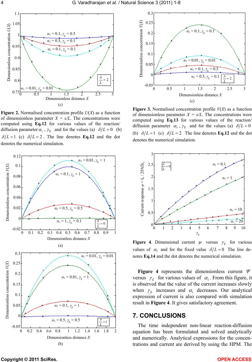 G. Varadharajan et al. / Natural Science 3 (2011) 1-8 Copyright © 2011 SciRes. OPEN ACCESS 4 Dimensionless distance X Dimensionless concentration U(X) α 1 = 0.1, γ E = 0.5 2 L δ α 1 = 0.5, γ E = 0.1 α 1 = 0.1, γ E = 0.1 α 1 = 0.01, γ E = 0.01 0 0.5 1 1.5 2 2.5 3 1.1 1.05 1 0.95 0.9 0.85 0.8 0.75 (c) Figure 2. Normalised concentration profile U(X) as a function of dimensionless parameter X = x/L. The concentrations were computed using Eq.12 for various values of the reaction/ diffusion parameter1E , and for the values (a) 0L (b) 1L (c) 2L . The line denotes Eq.12 and the dot denotes the numerical simulation. Dimensionless distance X Dimensionless concentration V(X) α 1 = 0.1, γ E = 1 0 L δ α 1 = 0.5, γ E = 0.5 α 1 = 1, γ E = 0.1 α 1 = 0.01, γ E = 1 0 0.1 0.2 0.3 0.4 0.5 0.6 0.7 0.8 0.9 1 0.12 0.1 0.08 0.06 0.04 0.02 0 -0.02 (a) Dimensionless distance X Dimensionless concentration V(X) α 1 = 0.01, γ E = 1 1 L δ α 1 = 0.1, γ E = 1 α 1 = 0.5, γ E = 0.5 α 1 = 0.01, γ E = 0.01 0 0.2 0.4 0.6 0.8 1 1.2 1.4 1.6 1.8 2 0.3 0.25 0.2 0.15 0.1 0.05 0 -0.05 (b) Dimensionless distance X Dimensionless concentration V(X) α 1 = 0.01, γ E = 0.01 2 L δ α 1 = 0.1, γ E = 0.5 α 1 = 0.5, γ E = 0.1 α 1 = 0.1, γ E = 0.1 0 0.5 1 1.5 2 2.5 3 0.3 0.25 0.2 0.15 0.1 0.05 0 -0.05 (c) Figure 3. Normalised concentration profile V(X) as a function of dimensionless parameter X = x/L. The concentrations were computed using Eq.13 for various values of the reaction/ diffusion parameter 1E , and for the values (a) 0L (b) 1L (c) 2L The line denotes Eq.12 and the dot denotes the numerical simulation. 0 L δ γ E α 1 = 0.1 0 1 2 3 4 5 6 7 8 9 10 3 2.5 2 1.5 1 0.5 0 α 1 = 1 α 1 = 10 α 1 = 20 Current response ψ = I a / 2FAD s ∞ Figure 4. Dimensional current versus E for various values of 1 and for the fixed value 0L The line de- notes Eq.14 and the dot denotes the numerical simulation. Figure 4 represents the dimensionless current versus E for various values of 1 . From this figure, it is observed that the value of the current increases slowly when E increases and 1 decreases. Our analytical expression of current is also compared with simulation result in Figure 4. It gives satisfactory agreement. 7. CONCLUSIONS The time independent non-linear reaction-diffusion equation has been formulated and solved analytically and numerically. Analytical expressions for the concen- trations and current are derived by using the HPM. The 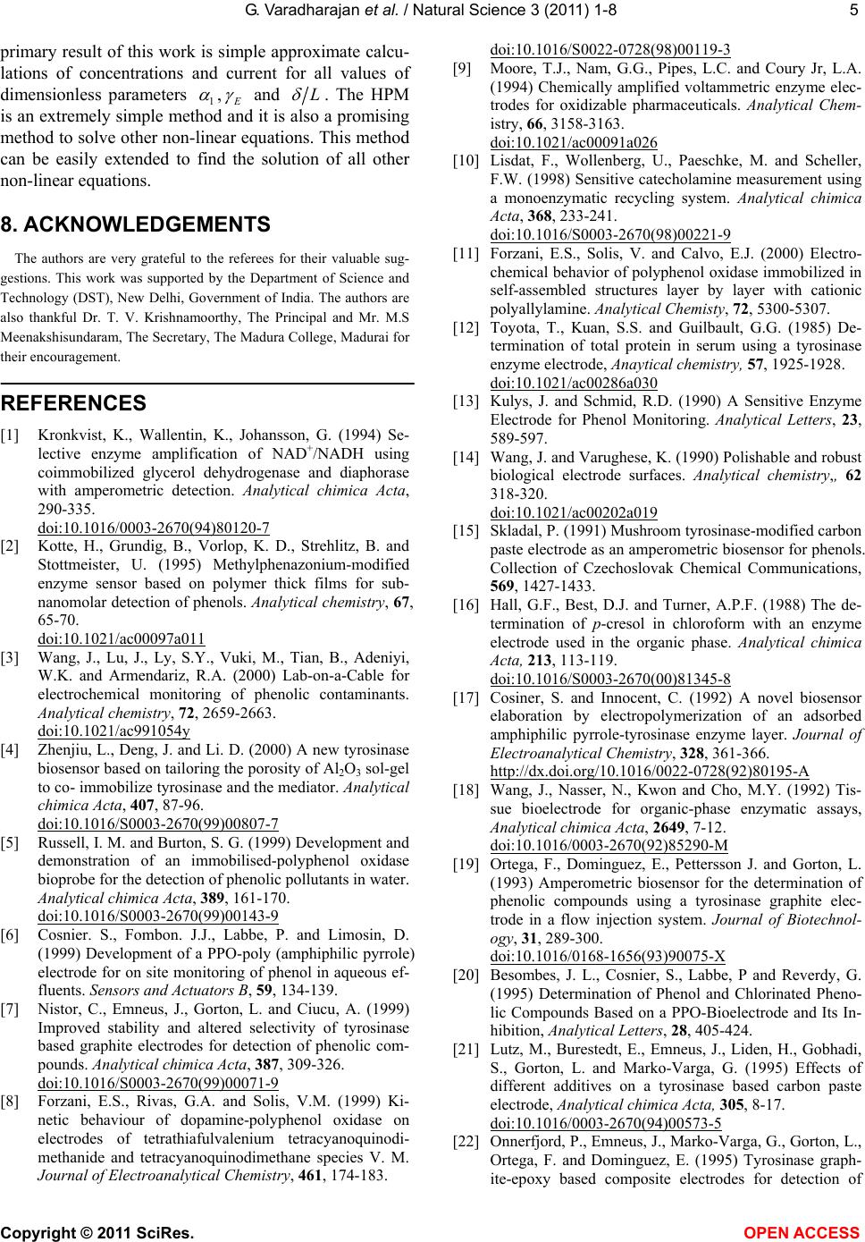 G. Varadharajan et al. / Natural Science 3 (2011) 1-8 Copyright © 2011 SciRes. OPEN ACCESS 55 primary result of this work is simple approximate calcu- lations of concentrations and current for all values of dimensionless parameters 1 , E and L . The HPM is an extremely simple method and it is also a promising method to solve other non-linear equations. This method can be easily extended to find the solution of all other non-linear equations. 8. ACKNOWLEDGEMENTS The authors are very grateful to the referees for their valuable sug- gestions. This work was supported by the Department of Science and Technology (DST), New Delhi, Government of India. The authors are also thankful Dr. T. V. Krishnamoorthy, The Principal and Mr. M.S Meenakshisundaram, The Secretary, The Madura College, Madurai for their encouragement. REFERENCES [1] Kronkvist, K., Wallentin, K., Johansson, G. (1994) Se- lective enzyme amplification of NAD+/NADH using coimmobilized glycerol dehydrogenase and diaphorase with amperometric detection. Analytical chimica Acta, 290-335. doi:10.1016/0003-2670(94)80120-7 [2] Kotte, H., Grundig, B., Vorlop, K. D., Strehlitz, B. and Stottmeister, U. (1995) Methylphenazonium-modified enzyme sensor based on polymer thick films for sub- nanomolar detection of phenols. Analytical chemistry, 67, 65-70. doi:10.1021/ac00097a011 [3] Wang, J., Lu, J., Ly, S.Y., Vuki, M., Tian, B., Adeniyi, W.K. and Armendariz, R.A. (2000) Lab-on-a-Cable for electrochemical monitoring of phenolic contaminants. Analytical chemistry, 72, 2659-2663. doi:10.1021/ac991054y [4] Zhenjiu, L., Deng, J. and Li. D. (2000) A new tyrosinase biosensor based on tailoring the porosity of Al2O3 sol-gel to co- immobilize tyrosinase and the mediator. Analytical chimica Acta, 407, 87-96. doi:10.1016/S0003-2670(99)00807-7 [5] Russell, I. M. and Burton, S. G. (1999) Development and demonstration of an immobilised-polyphenol oxidase bioprobe for the detection of phenolic pollutants in water. Analytical chimica Acta, 389, 161-170. doi:10.1016/S0003-2670(99)00143-9 [6] Cosnier. S., Fombon. J.J., Labbe, P. and Limosin, D. (1999) Development of a PPO-poly (amphiphilic pyrrole) electrode for on site monitoring of phenol in aqueous ef- fluents. Sensors and Actuators B, 59, 134-139. [7] Nistor, C., Emneus, J., Gorton, L. and Ciucu, A. (1999) Improved stability and altered selectivity of tyrosinase based graphite electrodes for detection of phenolic com- pounds. Analytical chimica Acta, 387, 309-326. doi:10.1016/S0003-2670(99)00071-9 [8] Forzani, E.S., Rivas, G.A. and Solis, V.M. (1999) Ki- netic behaviour of dopamine-polyphenol oxidase on electrodes of tetrathiafulvalenium tetracyanoquinodi- methanide and tetracyanoquinodimethane species V. M. Journal of Electroanalytical Chemistry, 461, 174-183. doi:10.1016/S0022-0728(98)00119-3 [9] Moore, T.J., Nam, G.G., Pipes, L.C. and Coury Jr, L.A. (1994) Chemically amplified voltammetric enzyme elec- trodes for oxidizable pharmaceuticals. Analytical Chem- istry, 66, 3158-3163. doi:10.1021/ac00091a026 [10] Lisdat, F., Wollenberg, U., Paeschke, M. and Scheller, F.W. (1998) Sensitive catecholamine measurement using a monoenzymatic recycling system. Analytical chimica Acta, 368, 233-241. doi:10.1016/S0003-2670(98)00221-9 [11] Forzani, E.S., Solis, V. and Calvo, E.J. (2000) Electro- chemical behavior of polyphenol oxidase immobilized in self-assembled structures layer by layer with cationic polyallylamine. Analytical Chemisty, 72, 5300-5307. [12] Toyota, T., Kuan, S.S. and Guilbault, G.G. (1985) De- termination of total protein in serum using a tyrosinase enzyme electrode, Anaytical chemistry, 57, 1925-1928. doi:10.1021/ac00286a030 [13] Kulys, J. and Schmid, R.D. (1990) A Sensitive Enzyme Electrode for Phenol Monitoring. Analytical Letters, 23, 589-597. [14] Wang, J. and Varughese, K. (1990) Polishable and robust biological electrode surfaces. Analytical chemistry,, 62 318-320. doi:10.1021/ac00202a019 [15] Skladal, P. (1991) Mushroom tyrosinase-modified carbon paste electrode as an amperometric biosensor for phenols. Collection of Czechoslovak Chemical Communications, 569, 1427-1433. [16] Hall, G.F., Best, D.J. and Turner, A.P.F. (1988) The de- termination of p-cresol in chloroform with an enzyme electrode used in the organic phase. Analytical chimica Acta, 213, 113-119. doi:10.1016/S0003-2670(00)81345-8 [17] Cosiner, S. and Innocent, C. (1992) A novel biosensor elaboration by electropolymerization of an adsorbed amphiphilic pyrrole-tyrosinase enzyme layer. Journal of Electroanalytical Chemistry, 328, 361-366. http://dx.doi.org/10.1016/0022-0728(92)80195-A [18] Wang, J., Nasser, N., Kwon and Cho, M.Y. (1992) Tis- sue bioelectrode for organic-phase enzymatic assays, Analytical chimica Acta, 2649, 7-12. doi:10.1016/0003-2670(92)85290-M [19] Ortega, F., Dominguez, E., Pettersson J. and Gorton, L. (1993) Amperometric biosensor for the determination of phenolic compounds using a tyrosinase graphite elec- trode in a flow injection system. Journal of Biotechnol- ogy, 31, 289-300. doi:10.1016/0168-1656(93)90075-X [20] Besombes, J. L., Cosnier, S., Labbe, P and Reverdy, G. (1995) Determination of Phenol and Chlorinated Pheno- lic Compounds Based on a PPO-Bioelectrode and Its In- hibition, Analytical Letters, 28, 405-424. [21] Lutz, M., Burestedt, E., Emneus, J., Liden, H., Gobhadi, S., Gorton, L. and Marko-Varga, G. (1995) Effects of different additives on a tyrosinase based carbon paste electrode, Analytical chimica Acta, 305, 8-17. doi:10.1016/0003-2670(94)00573-5 [22] Onnerfjord, P., Emneus, J., Marko-Varga, G., Gorton, L., Ortega, F. and Dominguez, E. (1995) Tyrosinase graph- ite-epoxy based composite electrodes for detection of  G. Varadharajan et al. / Natural Science 3 (2011) 1-8 Copyright © 2011 SciRes. OPEN ACCESS 6 phenols, Biosensors Bioelectronics, 10, 607-619. doi:10.1016/0956-5663(95)96937-T [23] Desprez, V. and Labbe, P. (1996) A Kinetic model for the electroenzymatic processd involved in polyphe- nol-oxidase- based amperometric catechol sensors. Journal of Electroanalytical Chemistry, 415, 191-195. doi:10.1016/S0022-0728(96)01011-X [24] Bartlett, P.N. and Whitaker, R.G. (1987) Electrochemi- cal immobilisation of enzymes: Part I. Theory, Journal of Electroanalytical Chemistry, 224, 27-35. doi:10.1016/0022-0728(87)85081-7 [25] Li, S.J. and Liu, Y.X. (2006) An improved approach to nonlinear dynamical system identification using PID neural networks,” International Journal of Nonlinear- Science and Numerical Simulation, 7, 177-182. [26] Mousa, M.M., Ragab, S.F. and Nturforsch, Z. (2008) Application of the homotopy perturbation method to lin- ear and nonlinear schrödinger equations, Zeitschrift für Naturforschung, 63, 140-144. [27] He, J.H, Homotopy perturbation technique, Computer Methods in Applied Mechanics and Engineering, vol. 178 (1999) 257-262. doi:10.1016/S0045-7825(99)00018-3 [28] He, J.H. (2003) Homotopy perturbation method: a new nonlinear analytical Technique. Applied Mathematics and Computation, 135, 73-79. doi:10.1016/S0096-3003(01)00312-5 [29] He, J.H. (2003) A Simple perturbation approach to Blasius equation”, Applied Mathematics and Computa- tion, 140, 217-222. doi:10.1016/S0096-3003(02)00189-3 [30] He, J.H. (2006) Some asymptotic methods for strongly nonlinear equations. International Journal of Modern Physics B, 20, 1141-1199. doi:10.1142/S0217979206033796 [31] He, J.H., Wu, G.C. and Austin, F. (2010) The variational iteration method which should be followed. Nonlinear Science Letters A, 1, 1-30. [32] He, J.H. (2000) A coupling method of a homotopy tech- nique and a perturbation technique for non-linear prob- lems. Internationl Journal of Nonlinear Mechanics, 35 37-43. doi:10.1016/S0020-7462(98)00085-7 [33] Ganji, D.D., Amini, M. and Kolahdooz, A. (2008) Ana- lytical investigation of hyperbolic Equations via He’s methods. American. Journal of Engineering and Applied Science, 1, 399-407. 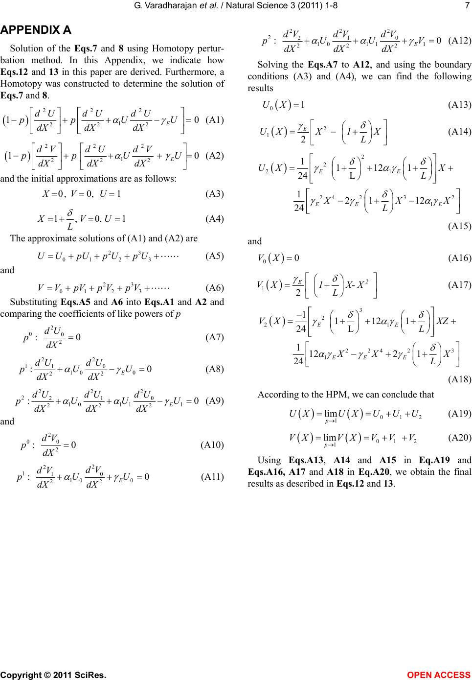 G. Varadharajan et al. / Natural Science 3 (2011) 1-8 Copyright © 2011 SciRes. OPEN ACCESS 77 APPENDIX A Solution of the Eqs.7 and 8 using Homotopy pertur- bation method. In this Appendix, we indicate how Eqs.12 and 13 in this paper are derived. Furthermore, a Homotopy was constructed to determine the solution of Eqs.7 and 8. 22 2 1 22 2 10 E dU dUdU ppUU dX dXdX (A1) 222 1 222 10 E dVdU dV ppUU dXdX dX (A2) and the initial approximations are as follows: 0, 0, 1XV U (A3) 1,0, 1XVU L (A4) The approximate solutions of (A1) and (A2) are 23 01 2 3 UUpU pUpU (A5) and 23 01 2 3 VVpV pVpV (A6) Substituting Eqs .A5 and A6 into Eqs.A1 and A2 and comparing the coefficients of like powers of p 2 00 2 : 0 dU pdX (A7) 2 2 10 1 10 0 22 :0 E dU dU pUU dX dX (A8) 2 22 20 21 10 111 222 :0 E dU dU dU pUUU dXdX dX (A9) and 2 00 2 : 0 dV pdX (A10) 2 2 10 1 10 0 22 : 0 E dV dV pUU dX dX (A11) 2 22 20 21 10 111 222 : 0 E dV dV dV pUUV dXdX dX (A12) Solving the Eqs.A7 to A12 , and using the boundary conditions (A3) and (A4), we can find the following results 01UX (A13) 2 12 E UXX 1X L (A14) 2 2 21 24 232 1 1 1121 24 L 1 2112 24 EE EE E UX X L X XX L (A15) and 00VX (A16) 12 2 E VX 1X- X L (A17) 3 2 21 224 23 1 1 1121 24 L 1 1221 24 EE EE E VX XZ L X XX L (A18) According to the HPM, we can conclude that 012 1 lim p UXUXUU U (A19) 01 2 1 lim p VXVXV VV (A20) Using Eqs.A13, A14 and A15 in Eq.A19 and Eqs.A16, A17 and A18 in Eq.A2 0, we obtain the final results as described in Eqs.12 and 13. 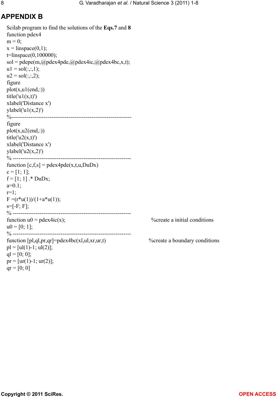 G. Varadharajan et al. / Natural Science 3 (2011) 1-8 Copyright © 2011 SciRes. OPEN ACCESS 8 APPENDIX B Scilab program to find the solutions of the Eqs.7 and 8 function pdex4 m = 0; x = linspace(0,1); t=linspace(0,100000); sol = pdepe(m,@pdex4pde,@pdex4ic,@pdex4bc,x,t); u1 = sol(:,:,1); u2 = sol(:,:,2); figure plot(x,u1(end,:)) title('u1(x,t)') xlabel('Distance x') ylabel('u1(x,2)') %--------------------------------------------------------------- figure plot(x,u2(end,:)) title('u2(x,t)') xlabel('Distance x') ylabel('u2(x,2)') % -------------------------------------------------------------- function [c,f,s] = pdex4pde(x,t,u,DuDx) c = [1; 1]; f = [1; 1] .* DuDx; a=0.1; r=1; F =(r*u(1))/(1+a*u(1)); s=[-F; F]; % -------------------------------------------------------------- function u0 = pdex4ic(x); %create a initial conditions u0 = [0; 1]; % -------------------------------------------------------------- function [pl,ql,pr,qr]=pdex4bc(xl,ul,xr,ur,t) %create a boundary conditions pl = [ul(1)-1; ul(2)]; ql = [0; 0]; pr = [ur(1)-1; ur(2)]; qr = [0; 0] |