Assessment of Profit of a Two-Stage Deteriorating Linear Consecutive 2-out-of-3 Repairable System

doi:10.4236/jamp.2013.13005

Paper Menu >>

Journal Menu >>

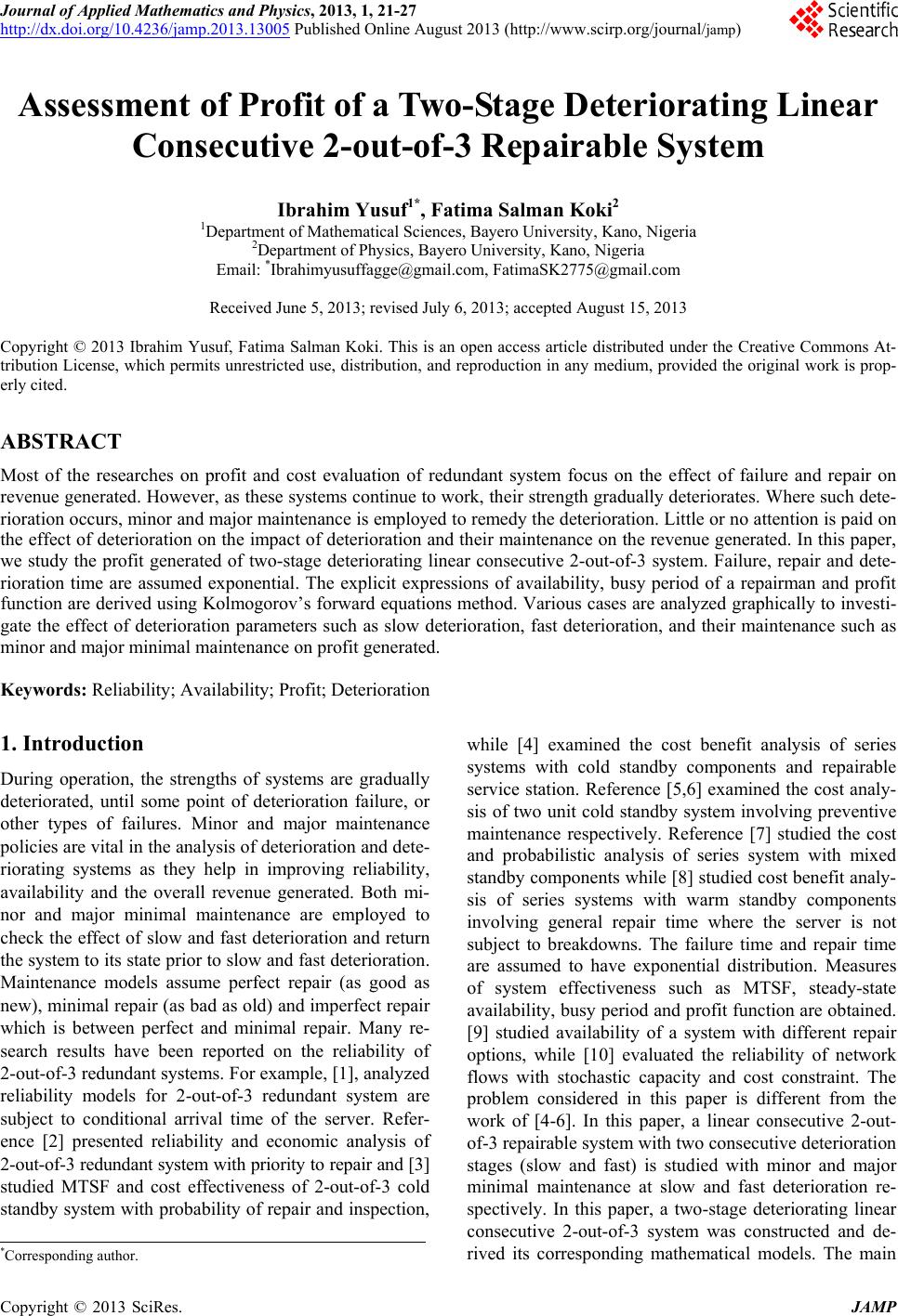Journal of Applied Mathematics and Physics, 2013, 1, 21-27

http://dx.doi.org/10.4236/jamp.2013.13005 Published Online August 2013 (http://www.scirp.org/journal/jamp)

Assessment of Profit of a Two-Stage Deteriorating Linear

Consecutive 2-out-of-3 Repairable System

Ibrahim Yusuf1*, Fatima Salman Koki2

1Department of Mathematical Sciences, Bayero University, Kano, Nigeria

2Department of Physics, Bayero University, Kano, Nigeria

Email: *[email protected]m, [email protected]

Received June 5, 2013; revised July 6, 2013; accepted August 15, 2013

tribution License, which permits unrestricted use, distribution, and reproduction in any medium, provided the original work is prop-

erly cited.

ABSTRACT

Most of the researches on profit and cost evaluation of redundant system focus on the effect of failure and repair on

revenue generated. However, as these systems continue to work, their strength gradually deteriorates. Where such dete-

rioration occurs, minor an d major maintenance is employed to remedy the deterioration . Little o r no attentio n is paid on

the effect of deterioration on the impact of deterioration and their maintenance on the revenue generated. In this paper,

we study the profit generated of two-stage deteriorating linear consecutive 2-out-of-3 system. Failure, repair and dete-

rioration time are assumed exponential. The explicit expressions of availability, busy period of a repairman and profit

function are derived using Kolmogorov’s forward equations method. Various cases are analyzed graphically to investi-

gate the effect of deterioration parameters such as slow deterioration, fast deterioration, and their maintenance such as

minor and major minimal maintenance on profit generated.

Keywords: Reliability; Availability; Profit; Deterioration

1. Introduction

During operation, the strengths of systems are gradually

deteriorated, until some point of deterioration failure, or

other types of failures. Minor and major maintenance

policies are vital in the analysis of deterioration and d ete-

riorating systems as they help in improving reliability,

availability and the overall revenue generated. Both mi-

nor and major minimal maintenance are employed to

check the effect of slow and fast deterioration and return

the system to its state prior to slow and fast deterioration.

Maintenance models assume perfect repair (as good as

new), minimal repair (as bad as old) and imperfect repair

which is between perfect and minimal repair. Many re-

search results have been reported on the reliability of

2-out-of-3 redu nd ant systems. For example, [1], analyzed

reliability models for 2-out-of-3 redundant system are

subject to conditional arrival time of the server. Refer-

ence [2] presented reliability and economic analysis of

2-out-of-3 redundant system with priority to repair and [3]

studied MTSF and cost effectiveness of 2-out-of-3 cold

standby system with probability of rep air and inspection,

while [4] examined the cost benefit analysis of series

systems with cold standby components and repairable

service station. Reference [5,6] examined the cost analy-

sis of two unit cold standby system involving preventive

maintenance respectively. Reference [7] studied the cost

and probabilistic analysis of series system with mixed

standby componen ts while [8] studied cost benefit analy-

sis of series systems with warm standby components

involving general repair time where the server is not

subject to breakdowns. The failure time and repair time

are assumed to have exponential distribution. Measures

of system effectiveness such as MTSF, steady-state

availability, busy p eriod and profit fun ction are obtained.

[9] studied availability of a system with different repair

options, while [10] evaluated the reliability of network

flows with stochastic capacity and cost constraint. The

problem considered in this paper is different from the

work of [4-6]. In this paper, a linear consecutive 2-out-

of-3 repairable system with two consecutive deterioration

stages (slow and fast) is studied with minor and major

minimal maintenance at slow and fast deterioration re-

spectively. In this paper, a two-stage deteriorating linear

consecutive 2-out-of-3 system was constructed and de-

rived its corresponding mathematical models. The main

*Corresponding author.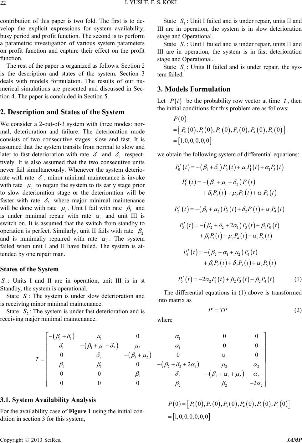

I. YUSUF, F. S. KOKI

contribution of this paper is two fold. The first is to de-

velop the explicit expressions for system availability,

busy period and profit function. The second is to perform

a parametric investigation of various system parameters

on profit function and capture their effect on the profit

function.

The rest of the paper is organized as follows. Section 2

is the description and states of the system. Section 3

deals with models formulation. The results of our nu-

merical simulations are presented and discussed in Sec-

tion 4. The paper is concluded in Section 5.

2. Description and States of the System

We consider a 2-out-of-3 system with three modes: nor-

mal, deterioration and failure. The deterioration mode

consists of two consecutive stages: slow and fast. It is

assumed that the system transits from normal to slow and

later to fast deterioration with rate 1



and 2



respect-

tively. It is also assumed that the two consecutive units

never fail simultaneously. Whenever the system deterio-

rate with rate 1



, minor minimal maintenance is invoke

with rate 1



to regain th e system to its early stage prior

to slow deterioration stage or the deterioration will be

faster with rate 2



where major minimal maintenance

will be done with rate 2



. Unit I fail with rate 1



and

is under minimal repair with rate 1



and unit III is

switch on. It is assumed that the switch from standby to

operation is perfect. Similarly, unit II fails with rate 2



and is minimally repaired with rate 2



. The system

failed when unit I and II have failed. The system is at-

tended by one repair man.

States of the System

0: Units I and II are in operation, unit III is in st

Standby, the system is operational.

State 1: The system is under slow deterioration and

is receiving minor minimal maintenance.

State 2: The system is under fast deterioration and is

receiving major minimal maintenance.

State 3: Unit I failed and is under repair, units II and

III are in operation, the system is in slow deterioration

stage and Operational.

State 4: Unit I failed and is under repair, units II and

III are in operation, the system is in fast deterioration

stage and Operational.

State 5: Units II failed and is under repair, the sys-

tem failed.

3. Models Formulation

Let





Pt be the probability row vector at time , then

the initial conditions for this problem are as follows:





  



012345

0,0, 0,0, 0,0

1,0,0,0,0,0

PPPPPP











we obtain the following system of differential equations:

 

0110111

PtPt Pt Pt

 

 3

 

11121

1022 13

Pt Pt

PtPt Pt





 



 

2122211

PtPt PtPt

 

 

 

 

322131

112 425

2PtPt Pt

Pt Pt Pt

 





 

 

 

42124

12 2325

Pt Pt

Pt PtPt





 



 

525232

2PtPt PtPt



 (1)

The differential equations in (1) above is transformed

into matrix as

PTP





(2)

where



11 11

11122 1

212 1

11 2212

12212

000

 



 

 











 

 



 



 



 



 



 

 

3.1. System Availability Analysis

For the availability case of Figure 1 using the initial con-

dition in section 3 for this system,































123456

0 0,0,0,0,0,0

1,0,0,0,0,0,0

P PPPPPP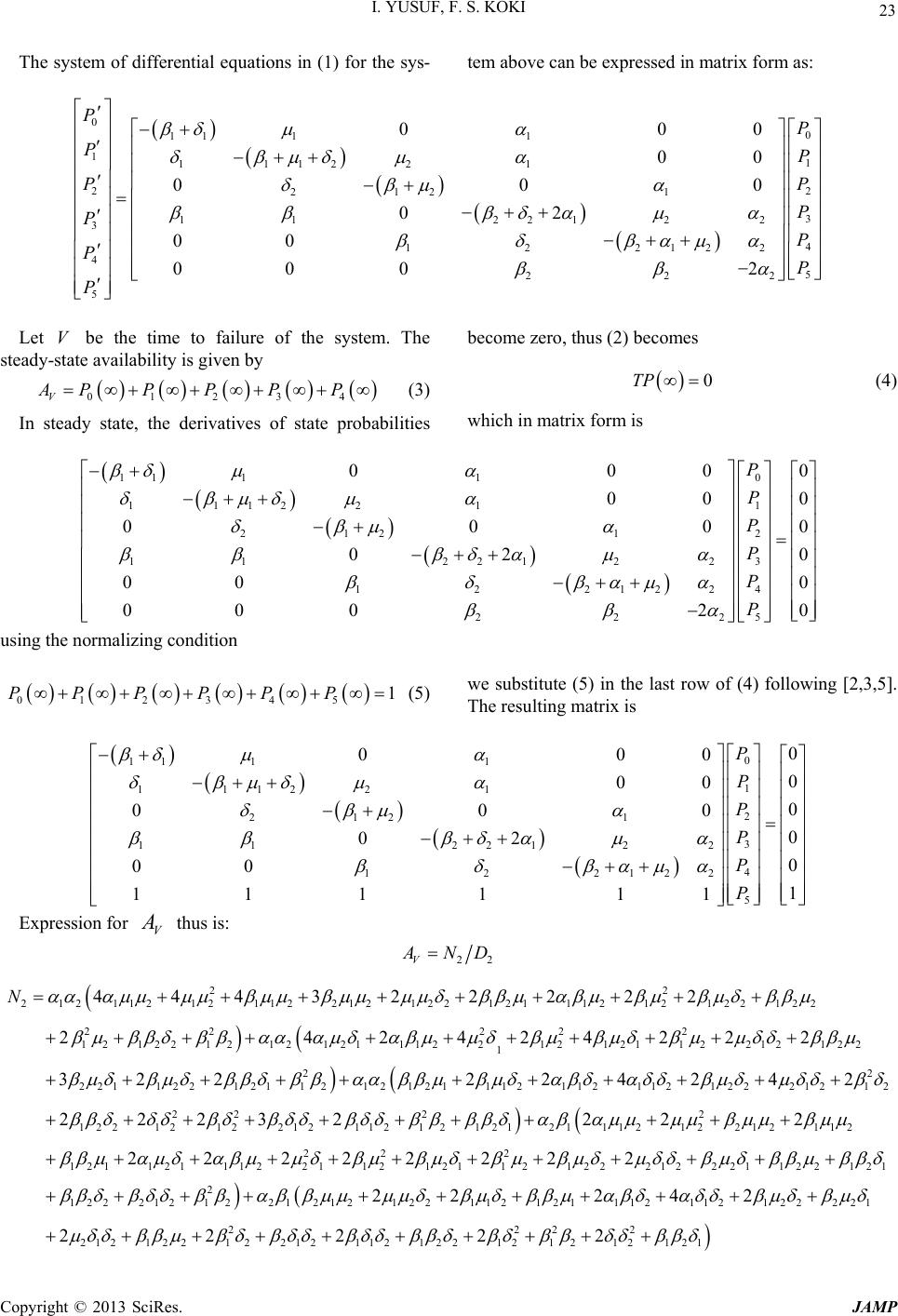











I. YUSUF, F. S. KOKI 23

The system of differential equations in (1) for the sys- tem above can be expressed in matrix form as:



11 11

111221

2 2

212 1

11 22122

122122

000 2

P P

 



 

 









  



 







 









  











 

 

 





 2

Let be the time to failure of the system. The

steady-state availability is given by

 





01234V

APP PPP



(3)

In steady state, the derivatives of state probabilities

become zero, thus (2) becomes





0TP



 (4)

which in matrix form is



11 11

11122 1

212 1

11 22122

122122

222

000 2

 



 

 







 

 



 

 

 



 



 





 



 

using the normalizing condition

 

012345

1PPPPPP (5) we substitute (5) in the last row of (4) following [2,3,5].

The resulting matrix is



11 11

11122 1

212 1

11 22122

122122

111 111

 

 

 

 



 

 



 

 

 



 



 



 



 

Expression for thus is:

22V









2 2

212112 12112 212 122 121112 12122122

22 222

1212212121211122 1212112212122

22112212112

444322222

24 2424 222

322

   

  

 

 

  







12121112 112 112 12221212

22 22

1221212212112121212111212212112

22 2

121 121 11221 121211212

224242

2223222 2

2222222



  

   





 

  







2212221 122121

1222121221212122 112121112 112 122221

2222

212122122121121 221212121 21

22 2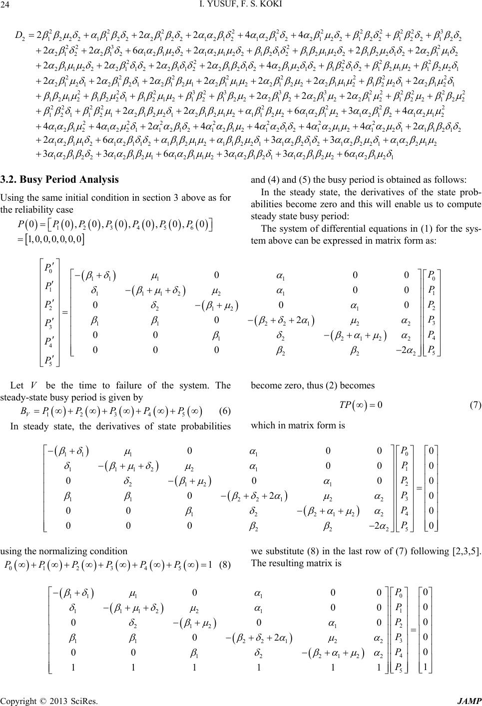42

22222



 

 





 



I. YUSUF, F. S. KOKI

22 222222223

212221122 212212121212 2122122122122

22 322

212212 12122 12122121212122 122122112

2112221

22244

22622 2































































 





 





 222

12211221 21221 2121 2 1212 121221

222 2 2222

21 2121 2121 2121122122211212212121

222323

1212122112121 21 22

22 4

22222 22







 



 









 



 

 

  

 

 3322222

2122122121221 22

22 222222

1 211 21212212121211 22121 2121 21212

22222 2

1212122112121212 1212 1212

222

2 2634

4424444









 

  





 



1221 11212

1211212112 1121211221122121222112212

12122 12121 12112 121211212212121

26 33

336336









      

       







3.2. Busy Period Analysis

Using the same initial condition in section 3 above as for

the reliability case































123456

0 0,0,0,0,0,0

1,0,0,0,0,0,0

PPPPPPP 





and (4) and (5) the busy period is obtain ed as follows:



In the steady state, the derivatives of the state prob-

abilities become zero and this will enable us to compute

steady state busy period:

The system of differential equations in (1) for the sys-

tem above can be expressed in matrix form as:



11 11

111221

2 2

212 1

11 22122

122122

000 2

P P

 

 

 

 









 

 



 







 









  











 

 

 







Let be the time to failure of the system. The

steady-state busy period is given by

 





12345V

BP PPPP



(6)

In steady state, the derivatives of state probabilities

become zero, thus (2) becomes





0TP



 (7)

which in matrix form is



11 11

11122 1

212 1

11 22122

122122

222

000 2

 

 

 

 







 

 



 

 

 



 



 





 



 

using the normalizing condition

 

012345

1PPPPPP (8) we substitute (8) in the last row of (7) following [2,3,5].

The resulting matrix is



11 11

11122 1

212 1

11 22122

12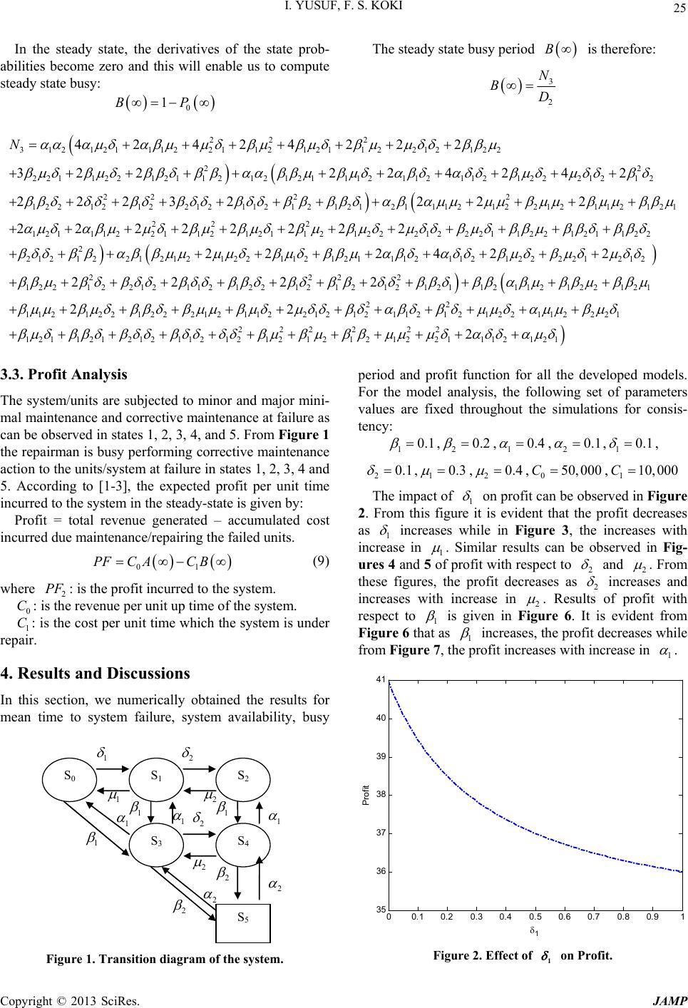2122

111 111

 

 

 

 













 

















 

I. YUSUF, F. S. KOKI 25

In the steady state, the derivatives of the state prob-

abilities become zero and this will enable us to compute

steady state busy:

 

1BP 

The steady state busy period is therefore:



B









22 2

312121 11221 1212112212122

2 2

221122 1211212121112 112112122212 12

22 2

122121221211212

42424222

322 224242

22232

  

   

 

 

 







1212111212212112 121

22 2

121112 2112 12112122 212221122121122

2121221212 122 112121112112

22 2

22222222

22 24





  

   



 

 

 



1 22221212

2222

1 22122121121 221212121 211 211 21221 21

112122 122212 112212 1211212 122 112221

22 22



    

     





 

 





222222

1121 212 112121212 12 1221112121

 

 

3.3. Profit Analysis

The system/units are subjected to minor and major mini-

mal maintenance and corrective maintenance at failure as

can be observed in states 1, 2, 3, 4, and 5. From Figure 1

the repairman is busy performing corrective maintenance

action to the units/system at failure in states 1, 2, 3, 4 and

5. According to [1-3], the expected profit per unit time

incurred to the system in the steady-state is giv e n by:

Profit = total revenue generated – accumulated cost

incurred due maintenance/repairing the failed units.

 

PFCAC B

(9)

where : is the profit incurred to the system.

: is the revenue per unit up time of the system.

C1: is the cost per unit time which the system is under

repair.

4. Results and Discussions

In this section, we numerically obtained the results for

mean time to system failure, system availability, busy































Figure 1. Transition diagram of the system.

period and profit function for all the developed models.

For the model analysis, the following set of parameters

values are fixed throughout the simulations for consis-

tency:

10.1





,20.2





,10.4





,20.1



,10.1





20.1





,10.3





,20.4





, ,

050,000C110,000C



The impact of 1



on profit can be observed in Figure

2. From this figure it is evident that the profit decreases

as 1



increases while in Figure 3, the increases with

increase in 1



. Similar results can be observed in Fig-

ures 4 and 5 of profit with respect to 2



and 2



. From

these figures, the profit decreases as 2



increases and

increases with increase in 2



. Results of profit with

respect to 1



is given in Figure 6. It is evident from

Figure 6 that as 1



increases, the profit decreases while

from Figure 7, the profit increases with increase in 1



00.1 0.20.3 0.40.5 0.6 0.70.8 0.9 1



Profit

Figure 2. Effect of 1



on Profit.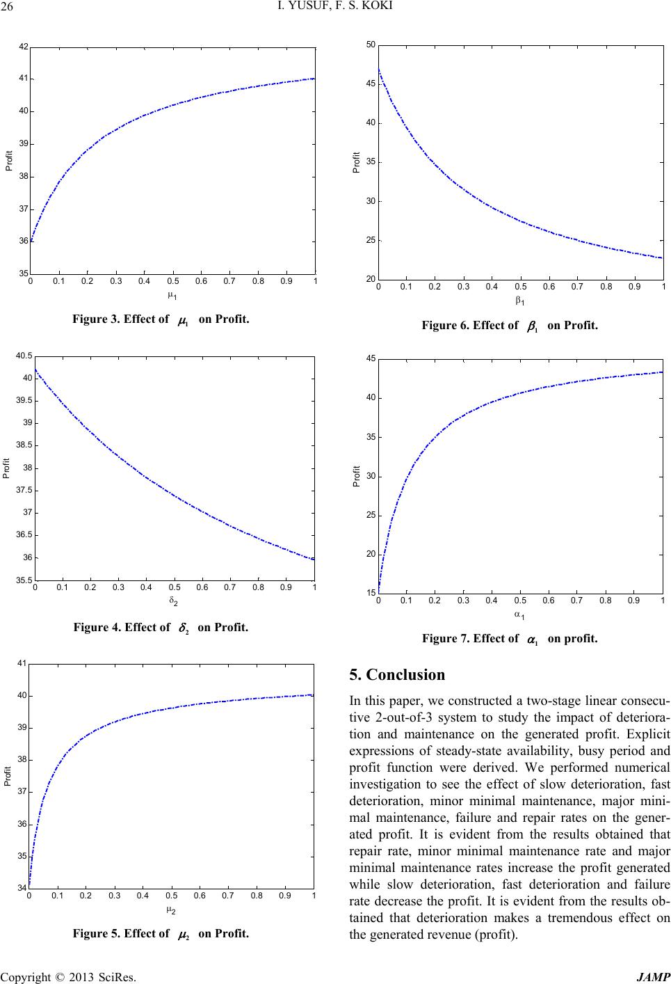

I. YUSUF, F. S. KOKI

00.1 0.20.3 0.40.5 0.6 0.70.8 0.91



Profit

Figure 3. Effect of 1



on Profit.

00.1 0.20.3 0.40.5 0.6 0.70.8 0.91

35. 5

36. 5

37. 5

38. 5

39. 5

40. 5



Profit

Figure 4. Effect of 2



on Profit.

00.1 0.20.3 0.40.5 0.6 0.70.8 0.91



Profit

Figure 5. Effect of 2



on Profit.

00.1 0.20.3 0.40.5 0.6 0.70.8 0.91



Profit

Figure 6. Effect of 1



on Profit.

00.1 0.20.3 0.40.5 0.6 0.70.8 0.91



Profit

Figure 7. Effect of 1



on profit.

5. Conclusion

In this paper, we constructed a two-stage linear consecu-

tive 2-out-of-3 system to study the impact of deteriora-

tion and maintenance on the generated profit. Explicit

expressions of steady-state availability, busy period and

profit function were derived. We performed numerical

investigation to see the effect of slow deterioration, fast

deterioration, minor minimal maintenance, major mini-

mal maintenance, failure and repair rates on the gener-

ated profit. It is evident from the results obtained that

repair rate, minor minimal maintenance rate and major

minimal maintenance rates increase the profit generated

while slow deterioration, fast deterioration and failure

rate decrease the profit. It is evident from the results ob-

tained that deterioration makes a tremendous effect on

the generated re venue ( pr ofit ) .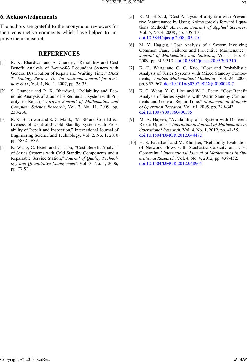

I. YUSUF, F. S. KOKI

6. Acknowledgements

The authors are grateful to the anonymous reviewers for

their constructive comments which have helped to im-

prove the manuscript.

REFERENCES

[1] R. K. Bhardwaj and S. Chander, “Reliability and Cost

Benefit Analysis of 2-out-of-3 Redundant System with

General Distribution of Repair and Waiting Time,” DIAS

Technology Review: The International Journal for Busi-

ness & IT, Vol. 4, No. 1, 2007, pp. 28-35.

[2] S. Chander and R. K. Bhardwai, “Reliability and Eco-

nomic Analysis of 2-out-of-3 Redundant System with Pri-

ority to Repair,” African Journal of Mathematics and

Computer Science Research, Vol. 2, No. 11, 2009, pp.

230-236.

[3] R. K. Bhardwai and S. C. Malik, “MTSF and Cost Effec-

tiveness of 2-out-of-3 Cold Standby System with Prob-

ability of Repair and Inspection,” International Journal of

Engineering Science and Technology, Vol. 2, No. 1, 2010,

pp. 5882-5889.

[4] K. Wang, C. Hsieh and C. Liou, “Cost Benefit Analysis

of Series Systems with Cold Standby Components and a

Repairable Service Station,” Journal of Quality Technol-

ogy and Quantitative Management, Vol. 3, No. 1, 2006,

pp. 77-92.

[5] K. M. El-Said, “Cost Analysis of a System with Preven-

tive Maintenance by Using Kolmogorov’s forward Equa-

tions Method,” American Journal of Applied Sciences,

Vol. 5, No. 4, 2008 , pp. 405-410.

doi:10.3844/ajassp.2008.405.410

[6] M. Y. Haggag, “Cost Analysis of a System Involving

Common Cause Failures and Preventive Maintenance,”

Journal of Mathematics and Statistics, Vol. 5, No. 4,

2009, pp. 305-310. doi:10.3844/jmssp.2009.305.310

[7] K. H. Wang and C. C. Kuo, “Cost and Probabilistic

Analysis of Series Systems with Mixed Standby Compo-

nents,” Applied Mathematical Modelling, Vol. 24, 2000,

pp. 957-967. doi:10.1016/S0307-904X(00)00028-7

[8] K. C. Wang, Y. C, Liou and W. L. Pearn, “Cost Benefit

Analysis of Series Systems with Warm Standby Compo-

nents and General Repair Time,” Mathematical Methods

of Operation Research, Vol. 61, 2005, pp. 329-343.

doi:10.1007/s001860400385

[9] M. A. Hajeeh, “Availability of a System with Different

Repair Options,” International Journal of Mathematics in

Operational Research, Vol. 4, No. 1, 2012, pp. 41-55.

doi:10.1504/IJMOR.2012.044472

[10] H. S. Fathabadi and M. Khodaei, “Reliability Evaluation

of Network Flows with Stochastic Capacity and Cost

Constraint,” International Journal of Mathematics in Op-

erational Research, Vol. 4, No. 4, 2012, pp. 439-452.

doi:10.1504/IJMOR.2012.048904