A Wireless Inductive-Capacitive Resonant Circuit Sensor Array for Force Monitoring

doi:10.4236/jst.2013.33011

Paper Menu >>

Journal Menu >>

Journal of Sensor Technology, 2013, 3, 63-69

http://dx.doi.org/10.4236/jst.2013.33011 Published Online September 2013 (http://www.scirp.org/journal/jst)

A Wireless Inductive-Capacitive Resonant Circuit

Sensor Array for Force Monitoring

Andrew J. DeRouin, Brandon D. Pereles, Thadeus M. Sansom, Peng Zang, Keat Ghee Ong

Department of Biomedical Engineering, Michigan Technological University, Houghton, USA

Email: [email protected]

Received July 11, 2013; revised August 11, 2013; accepted August 19, 2013

cense, which permits unrestricted use, distribution, and reproduction in any medium, provided the original work is properly cited.

ABSTRACT

A wireless passive sensor array based on inductive-cap acitive (LC) resonant circuits capable of simultan eously tracking

two points of force loading is described. The sensor consisted of a planar spiral inductor connected to two capacitors

forming a resonant circuit with two resonant frequencies. When a load was applied to one or both of the parallel plate

capacitors, the distance between the plates of the capacitor was altered, thus shifting the observed resonant peaks. Test-

ing illustrated that applied loading to a particular capacitor caused a significant shift in one of the resonant peaks and

also a smaller shift in another resonant peak. This interdependence resulted from each capacitive element being con-

nected to the same inductive spiral and was accounted for with a developed analysis algorithm. To validate the experi-

mental observation, a circuit simulation was also generated to model the sensor behavior with changing force/displace-

ment. The novelty of this syste m lies not only in its wireless passive nature, bu t also in the fact that a single LC sensor

was fashioned to detect more than one point simul taneously.

Keywords: Force Sensors; RFID Tags; Sensor Array; Wireless Sensors

1. Introduction

Generally, wireless sensors consist of sensor components

for taking local measurements placed at the areas of in-

terest and a remotely located system to receive informa-

tion wirelessly for processing and presentation [1-3].

Since these systems lack physical connections between

the sensing components and the processing apparatus,

they are highly versatile in terms of sensor deployment,

and are thus ideal for wide area monitoring. Additionally,

wireless sensors have the capacity to operate, depending

on the particular method of data acquisition and trans-

mission, in an active or passive mode. Active sensors are

powered with an internal source whereas passive devices

receive power remotely. While active wireless sensors

can monitor a wide range of parameters encompassing a

large region, they can also suffer from significant instal-

lation and maintenance costs and battery lifetime limita-

tions [4]. Passive wireless sensors, on the other hand,

have limited functionality compared to their active coun-

terparts but are generally cheaper, easier to implement

and last longer. There are many types of wireless passive

sensors, and most of them are powered magnetically or

electromagnetically. Examples of these sensors include

magnetoelastic, inductive-capacitive, and surface acous-

tic sensors [5-9].

A wireless passive sensor, known as the inductive-

capacitive (LC) sensor, was developed to monitor chang-

ing environmental conditions such as temperature, hu-

midity and pressure [10]. This type of sensor altered its

capacitance depending on the experienced environmental

parameter, resulting in a shift in its resonant frequency.

The change in resonant frequenc y was remotely captured

with a coil antenna by monitoring its impedance change

[10]. Unfortunately, the limitation of the existing LC

sensors is their inability to monitor multiple parameters.

For applications that require simultaneous detection of

multiple targets, more than one LC sensor is necessary,

significantly increasing the overall sensor size with no

improvement to sensor detection range. Therefore, a two

element sensor was developed comprised of a planar

square spiral inductor and two parallel plate capacitors.

While the operating principle of the presented sensor

is the same as current LC sensor technologies [10], it

features multiple sensing elements (capacitors) sharing

the same inductor. As a result, there are interferences

among the capacitive elements and further investigations

were performed to realize the new, two-element sensor

design.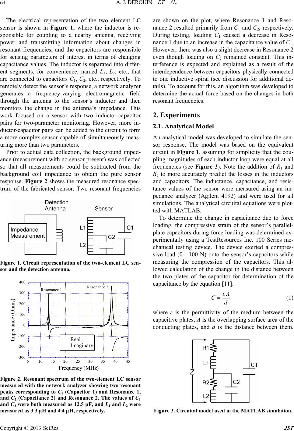

A. J. DEROUIN ET AL.

The electrical representation of the two element LC

sensor is shown in Figure 1, where the inductor is re-

sponsible for coupling to a nearby antenna, receiving

power and transmitting information about changes in

resonant frequencies, and the capacitors are responsible

for sensing parameters of interest in terms of changing

capacitance values. The inductor is separated into differ-

ent segments, for convenience, named L1, L2, etc., that

are connected to capacitors C1, C2, etc., respectively. To

remotely detect the sensor’s response, a network analyzer

generates a frequency-varying electromagnetic field

through the antenna to the sensor’s inductor and then

monitors the change in the antenna’s impedance. This

work focused on a sensor with two inductor-capacitor

pairs for two-parameter monitoring. However, more in-

ductor-capacitor pairs can be added to the circu it to form

a more complex sensor capable of simultaneously meas-

uring more than two parameters.

Prior to actual data collection, the background imped-

ance (measurement with no sensor present) was collected

so that all measurements could be subtracted from the

background coil impedance to obtain the pure sensor

response. Figure 2 shows the measured resonance spec-

trum of the fabricated sensor. Two resonant frequencies

Figure 1. Circuit representation of the two-element LC sen-

sor and the detection antenna.

-300

-200

-100

100

200

300

400

5 1015202530354045

Real

Imaginary

Impedanc e (O hms)

Frequency (MHz)

Resonance 1Resonance 2

Figure 2. Resonant spectrum of the two-element LC sensor

measured with the network analyzer showing two resonant

peaks corresponding to C1 (Capacitor 1) and Resonance 1,

and C2 (Capacitance 2) and Resonance 2. The values of C1

and C2 were both measured as 12.5 pF, and L1 and L2 were

measured as 3.3 µH and 4.4 µH, respectively.

are shown on the plot, where Resonance 1 and Reso-

nance 2 resulted primarily from C1 and C2, respectively.

During testing, loading C1 caused a decrease in Reso-

nance 1 due to an increase in the capacitance value of C1.

However, there was also a slight decrease in Resonance 2

even though loading on C2 remained constant. This in-

terference is expected and explained as a result of the

interdependence between capacitors physically connected

to one inductive spiral (see discussion for additional de-

tails). To account for this, an algorithm was developed to

determine the actual force based on the changes in both

resonant frequencies.

2. Experiments

2.1. Analytical Model

An analytical model was developed to simulate the sen-

sor response. The model was based on the equivalent

circuit in Figure 1, assuming for simplicity that the cou-

pling magnitudes of each inductor loop were equal at all

frequencies (see Figure 3). Note the addition of R1 and

R2 to more accurately predict the losses in the inductors

and capacitors. The inductance, capacitance, and resis-

tance values of the sensor were measured using an im-

pedance analyzer (Agilent 4192) and were used for all

simulations. The analytical circuital equations were plot-

ted with MATLAB.

To determine the change in capacitance due to force

loading, the compressive strain of the sensor’s parallel-

plate capacitors during force loading was determined ex-

perimentally using a TestResources Inc. 100 Series me-

chanical testing device. The device exerted a compres-

sive load (0 - 100 N) onto the sensor’s capacitors while

measuring the compression of the capacitors. This al-

lowed calculation of the change in the distance between

the two plates of the capacitor for determination of the

capacitance by the equation [11]:



 (1)

where ε is the permittivity of the medium between the

capacitive plates, A is the overlapping surface area of the

conducting plates, and d is the distance between them.

Figure 3. Circuital model used in the MATLAB simulation.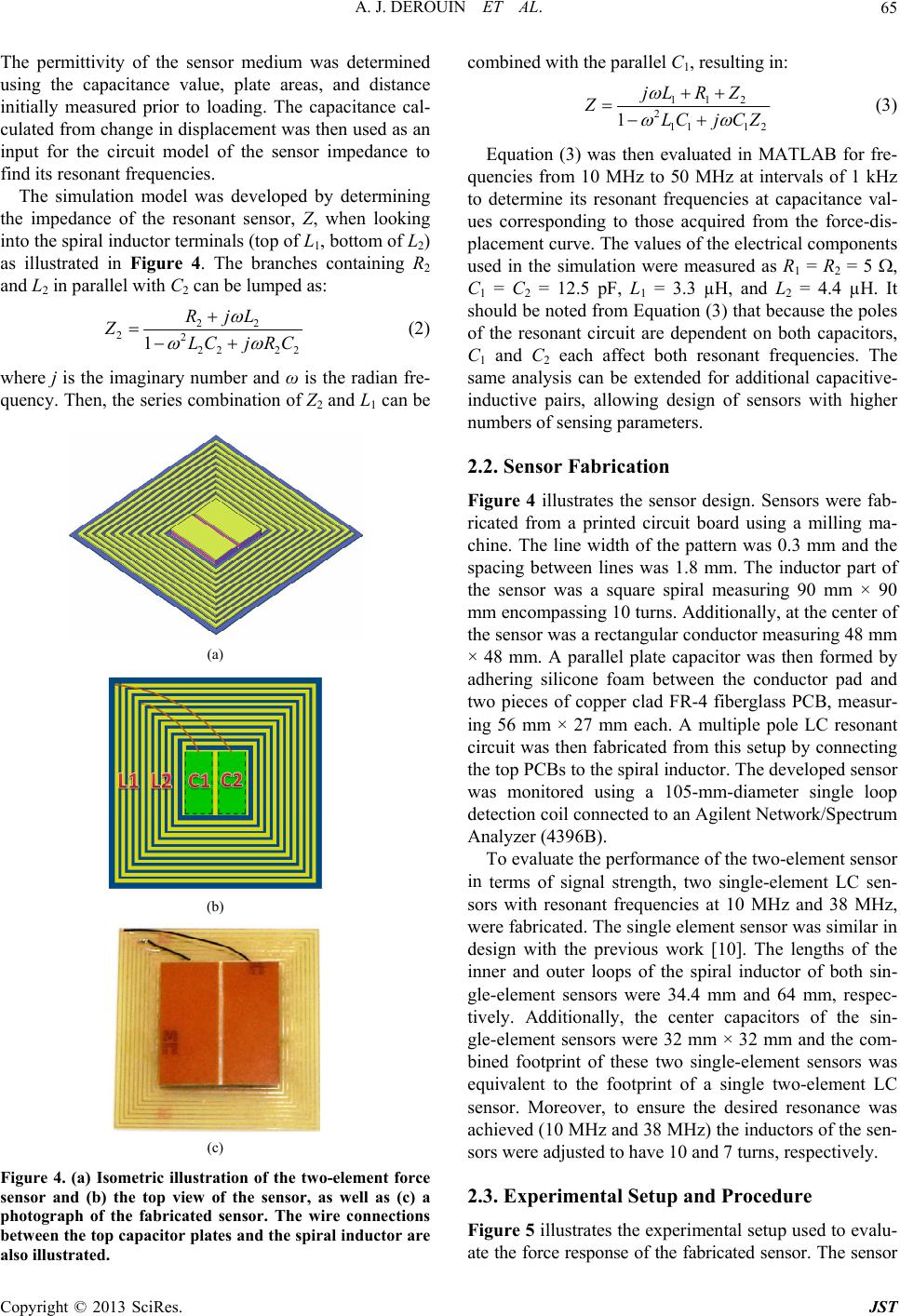

A. J. DEROUIN ET AL. 65

The permittivity of the sensor medium was determined

using the capacitance value, plate areas, and distance

initially measured prior to loading. The capacitance cal-

culated from change in displacement was then used as an

input for the circuit model of the sensor impedance to

find its resonant frequencies.

The simulation model was developed by determining

the impedance of the resonant sensor, Z, when looking

into the spiral inductor terminals (top of L1, bottom of L2)

as illustrated in Figure 4. The branches containing R2

and L2 in parallel with C2 can be lumped as:

2222 22

RjL

ZLCj RC









 (2)

where j is the imaginary number and ω is the radian fre-

quency. Then, the series combination of Z2 and L1 can be

(a)

(b)

(c)

Figure 4. (a) Isometric illustration of the two-element force

sensor and (b) the top view of the sensor, as well as (c) a

photograph of the fabricated sensor. The wire connections

between the top capacitor plates and the spir al inductor are

combined with th

also illustrated.

e parallel C, resulting in:

112

211 12

jL R Z





ZLC j CZ





 (3)

Equation (3) was then evaluated in MATLAB for fre-

2.2. Sensor Fabrication

or design. Sensors were fab-

rformance of the two-element sensor

2.3. Experimental Setup and Procedure

to evalu-

encies from 10 MHz to 50 MHz at intervals of 1 kHz

to determine its resonant frequencies at capacitance val-

ues corresponding to those acquired from the force-dis-

placement curve. The values of the electrical components

used in the simulation were measured as R1 = R2 = 5 ,

C1 = C2 = 12.5 pF, L1 = 3.3 µH, and L2 = 4.4 µH. It

should be noted from Equation (3) that because the poles

of the resonant circuit are dependent on both capacitors,

C1 and C2 each affect both resonant frequencies. The

same analysis can be extended for additional capacitive-

inductive pairs, allowing design of sensors with higher

numbers of sensing parameters.

Figure 4 illustrates the sens

ricated from a printed circuit board using a milling ma-

chine. The line width of the pattern was 0.3 mm and the

spacing between lines was 1.8 mm. The inductor part of

the sensor was a square spiral measuring 90 mm × 90

mm encompassing 10 turns. Addition ally, at the cen ter of

the sensor was a rectangular condu ctor measuring 48 mm

× 48 mm. A parallel plate capacitor was then formed by

adhering silicone foam between the conductor pad and

two pieces of copper clad FR-4 fiberglass PCB, measur-

ing 56 mm × 27 mm each. A multiple pole LC resonant

circuit was then fabricated from this setup by connecting

the top PCBs to the spiral inductor. The developed sensor

was monitored using a 105-mm-diameter single loop

detection coil co nnected to an Agilent Network/Sp ectrum

Analyzer (4396B).

To evaluate the pe

terms of signal strength, two single-element LC sen-

sors with resonant frequencies at 10 MHz and 38 MHz,

were fabricated. The single element sensor was similar in

design with the previous work [10]. The lengths of the

inner and outer loops of the spiral inductor of both sin-

gle-element sensors were 34.4 mm and 64 mm, respec-

tively. Additionally, the center capacitors of the sin-

gle-element sensors were 32 mm × 32 mm and the com-

bined footprint of these two single-element sensors was

equivalent to the footprint of a single two-element LC

sensor. Moreover, to ensure the desired resonance was

achieved (10 MHz and 38 MHz) the inducto rs of the sen-

sors were adjusted to have 10 and 7 turns, respectively.

Figure 5 illustrates the experimental setup used

ate the force response of the fabricated sensor. The sensor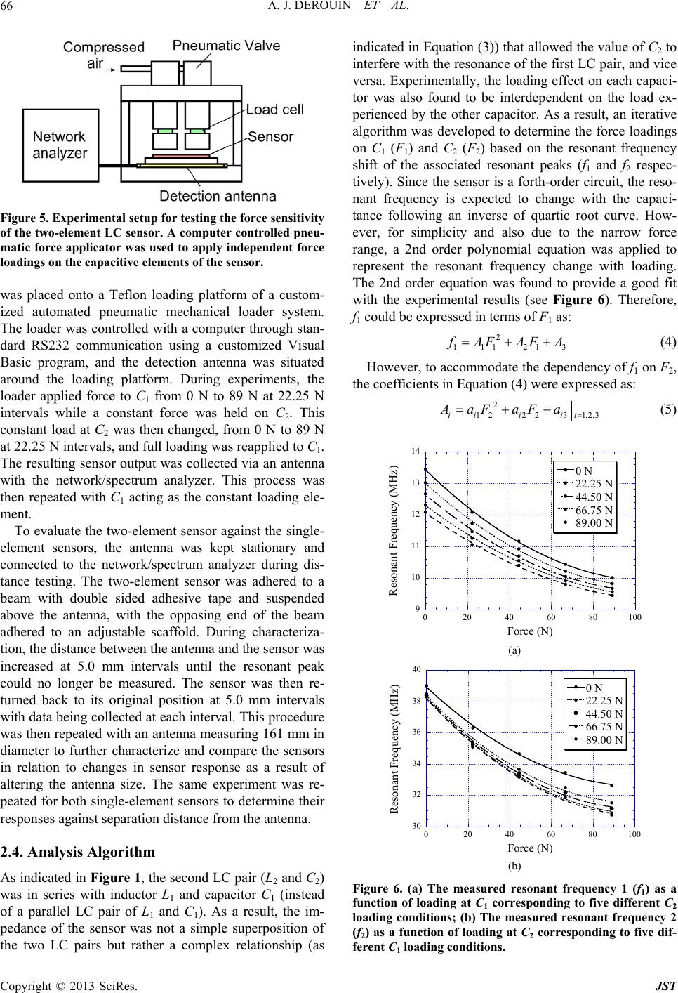

A. J. DEROUIN ET AL.

Figure 5. Experimental setup fo r testing the force sensity

as placed onto a Teflon loading platform of a custom-

valuate the two-element sensor against the single-

2.4. Analysis Algorithm

second LC pair (L2 and C2)

ivit

of the two-element LC sensor. A computer controlled pneu-

matic force applicator was used to apply independent force

loadings on the capacitive elements of the sensor.

ized automated pneumatic mechanical loader system.

The loader was controlled with a computer through stan-

dard RS232 communication using a customized Visual

Basic program, and the detection antenna was situated

around the loading platform. During experiments, the

loader applied force to C1 from 0 N to 89 N at 22.25 N

intervals while a constant force was held on C2. This

constant load at C2 was then changed, from 0 N to 89 N

at 22.25 N intervals, and full loading was reapplied to C1.

The resulting sensor output was collected via an antenna

with the network/spectrum analyzer. This process was

then repeated with C1 acting as the constant loading ele-

ment.

To e

ement sensors, the antenna was kept stationary and

connected to the network/spectrum analyzer during dis-

tance testing. The two-element sensor was adhered to a

beam with double sided adhesive tape and suspended

above the antenna, with the opposing end of the beam

adhered to an adjustable scaffold. During characteriza-

tion, the distance between the antenna and the sensor was

increased at 5.0 mm intervals until the resonant peak

could no longer be measured. The sensor was then re-

turned back to its original position at 5.0 mm intervals

with data being collected at each interval. This procedure

was then repeated with an antenna measuring 161 mm in

diameter to further characterize and compare the sensors

in relation to changes in sensor response as a result of

altering the antenna size. The same experiment was re-

peated for both single-element sensors to determine their

responses against separation distance from the antenna.

As indicated in Figure 1, the

was in series with inductor L1 and capacitor C1 (instead

of a parallel LC pair of L1 and C1). As a result, the im-

pedance of the sensor was not a simple superposition of

the two LC pairs but rather a complex relationship (as

indicated in Equation (3)) that allowed the value of C2 to

interfere with the resonance of the first LC pair, and vice

versa. Experimentally, the loading effect on each capaci-

tor was also found to be interdependent on the load ex-

perienced by the other capacitor. As a result, an iterative

algorithm was developed to determine the force loadings

on C1 (F1) and C2 (F2) based on the resonant frequency

shift of the associated resonant peaks (f1 and f2 respec-

tively). Since the sensor is a forth-order circuit, the reso-

nant frequency is expected to change with the capaci-

tance following an inverse of quartic root curve. How-

ever, for simplicity and also due to the narrow force

range, a 2nd order polynomial equation was applied to

represent the resonant frequency change with loading.

The 2nd order equation was found to provide a good fit

with the experimental results (see Figure 6). Therefore,

f1 could be expressed in terms of F1 as:

111 21

AFA FA



 (4)

However, to accommodate the depe1 2

th ndency of f on F,

e coefficients in Equatio n (4) were expressed as:

AaFaFa

12 223 1,2,3iii ii (5)

0 20406080100

0 N

22.25 N

44.50 N

66.75 N

89.00 N

Resonant Frequency (MHz)

Force (N)

(a)

020406080100

0 N

22.25 N

44.50 N

66.75 N

89.00 N

Resonant Frequency (MHz)

Force (N)

(b)

Figure 6. (a) The measuredonant frequency 1 (f1) as a

res

function of loading at C1 corresponding to five different C2

loading conditions; (b) The measured resonant frequency 2

(f2) as a function of loading at C2 corresponding to five dif-

ferent C loading conditions.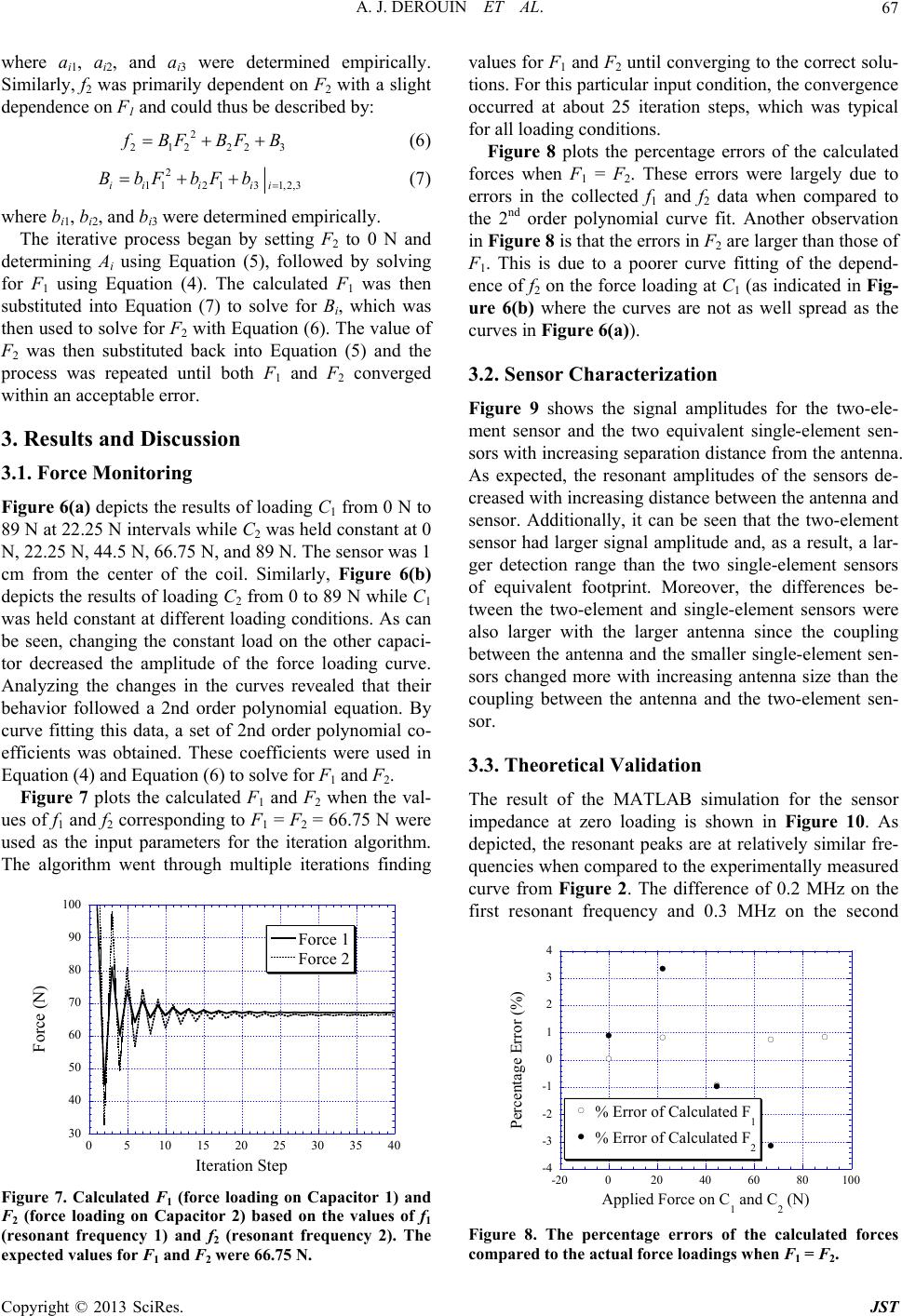

A. J. DEROUIN ET AL. 67

where ai1, ai2, and ai3 were determined empirically.

Similarly, f2 was primarily dependent on F2 with a slight

dependence on F1 and could thus be described by:

212 223

BFB FB (6)

11213 1,2,3

(7)

ii i ii

BbF bFb





where bi1, bi2, and bi3 were determined e

te i and

ults of loading C1 from 0 N to

mpirically.

The iratve process began by setting F2 to 0 N

determining A using Equation (5), followed by so

ilving

for F1 using Equation (4). The calculated F1 was then

substituted into Equation (7) to solve for Bi, which was

then used to solve for F2 with Equation (6). The value of

F2 was then substituted back into Equation (5) and the

process was repeated until both F1 and F2 converged

within an acceptab le error.

3. Results and Discussi

3.1. Force Monitoring

Figure 6(a) depicts the res

89 N at 22.25 N intervals while C2 was heldnstant at 0

N, 22.25 N, 44.5 N, 66 .75 N , and 8 9 N . Th e senso r was 1

cm from the center of the coil. Similarly, Figure 6(b)

depicts the resu lts of loading C2 from 0 to 89 N while C1

was held constant at different loading conditions. As can

be seen, changing the constant load on the other capaci-

tor decreased the amplitude of the force loading curve.

Analyzing the changes in the curves revealed that their

behavior followed a 2nd order polynomial equation. By

curve fitting this data, a set of 2nd order polynomial co-

efficients was obtained. These coefficients were used in

Equation (4) and Eq uation (6) to solve for F1 and F2.

Figure 7 plots the calculated F1 and F2 when the val-

ues of f and f corresponding to F1 = F = 66.75 N w

1 22ere

used as the input parameters for the iteration algorithm.

The algorithm went through multiple iterations finding

100

0510 15 20 25 30 35 40

Force 1

Force 2

Force (N)

Iteration Step

Figure 7. Calculated F1 (force loading on Capacitor 1)nd

F (force loading on Capacitor 2) based on the values of f

expected values for F1 and F2 were 66.75 N.

Figure 9 shows the signal amplitudes for the two-ele-

nt single-element sen-

The result of the MATLAB simulation for the sensor

hown in Figure 10. As

2 1

(resonant frequency 1) and f2 (resonant frequency 2). The

values for F1 and F2 until converging to the correct solu-

tions. For this particular input condition, th e convergence

occurred at about 25 iteration steps, which was typical

for all loading conditions.

Figure 8 plots the percentage errors of the calculated

forces when F1 = F2. These errors were largely due to

errors in the collected f1 and f2 data when compared to

the 2nd order polynomial curve fit. Another observation

in Figure 8 is that the errors in F2 are larger than those of

F1. This is due to a poorer curve fitting of the depend-

ence of f2 on the force loading at C1 (as indicated in Fig-

ure 6(b) where the curves are not as well spread as the

curves in Figure 6(a)).

3.2. Sensor Characterization

ment sensor and the two equivale

sors with increasing sepa ration distance from the antenn a.

As expected, the resonant amplitudes of the sensors de-

creased with increasing distance between the antenna and

sensor. Additionally, it can be seen that the two-element

sensor had larger signal amplitude and, as a result, a lar-

ger detection range than the two single-element sensors

of equivalent footprint. Moreover, the differences be-

tween the two-element and single-element sensors were

also larger with the larger antenna since the coupling

between the antenna and the smaller single-element sen-

sors changed more with increasing antenna size than the

coupling between the antenna and the two-element sen-

sor.

3.3. Theoretical Validation

impedance at zero loading is s

depicted, the resonant peaks are at relatively similar fre-

quencies when compared to the experimentally measured

curve from Figure 2. The difference of 0.2 MHz on the

first resonant frequency and 0.3 MHz on the second

-4

-3

-2

-1

% Error of Calculated F

-20 020 40 60 80100

% Error of Calculated F

Percentage Error (%)

Applied Force on C

and C

(N)

Figure 8. The percentage errors of the calculated forces

compared to the actual force loadings when F1 = F2.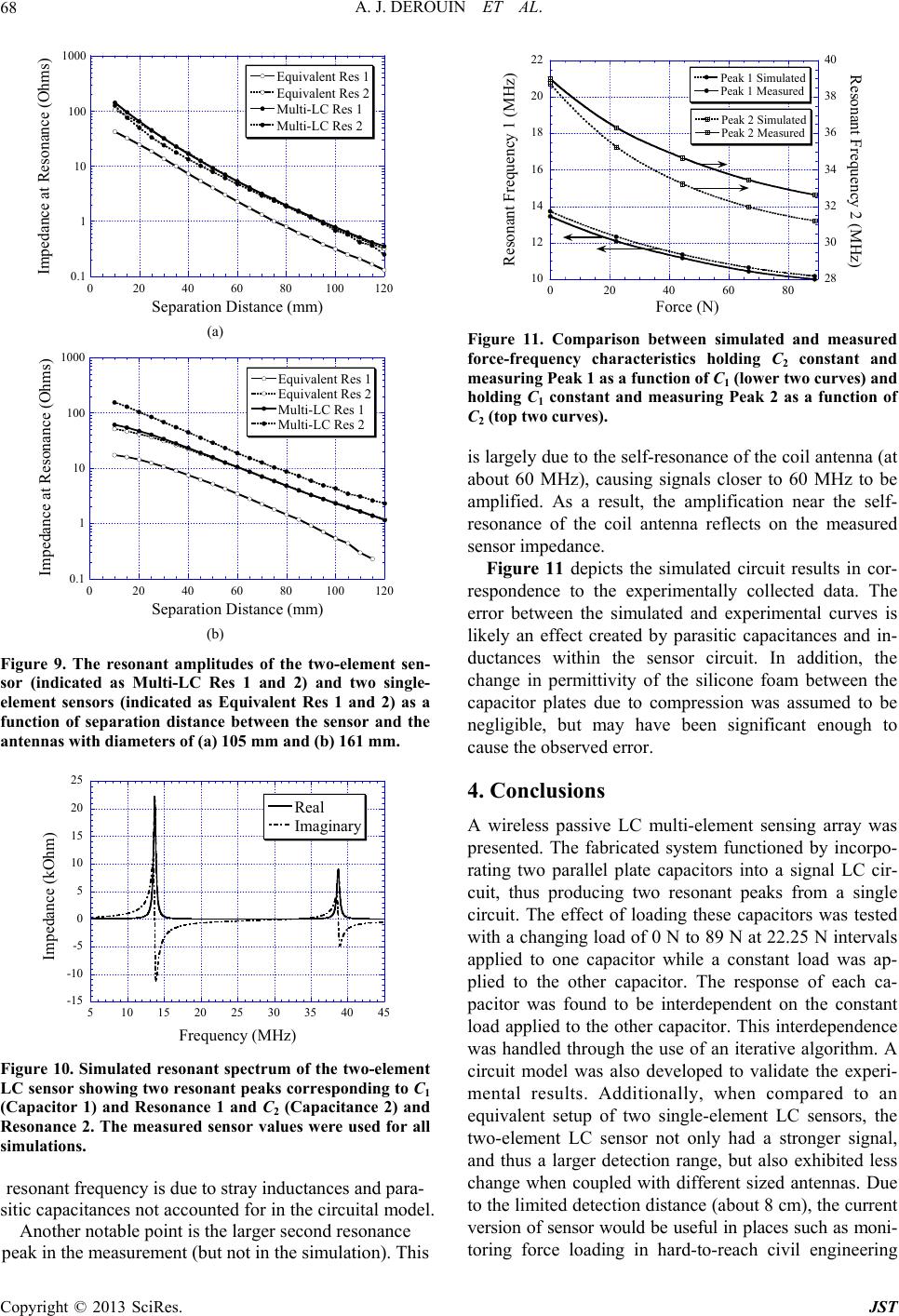

A. J. DEROUIN ET AL.

0.1

100

1000

0 20406080100120

Equivalent Res 1

Equivalent Res 2

Multi- L C Res 1

Multi- L C Res 2

Impedance at Resonance (Ohms)

Separation Distance (mm)

(a)

0.1

100

1000

020 40 60 80100120

Equivalent Res 1

Equivalent Res 2

Multi-LC Res 1

Multi-LC Res 2

Impedance at Resonance (Ohm

Separation Distance ( mm)

(b)

Figure 9. The resonant ampdes of the two-element sen-

sor (indicated as Multi-LC Res 1 and 2) and two single-

element sensors (indicated as Equivalent Res 1 and 2) as a

function of separation distance between the sensor and the

antennas with diameters of (a) 105 mm and (b) 161 mm.

litu

-15

-10

5 1015202530354045

-5

Real

Imaginary

Impedance (kOhm)

ent

C sensor showing two resonant peaks corresponding to C1

(Capacitor 1) and Resonance 1 and C2 (Capacitance 2) and

Resonance 2. The measured sensor values were used for all

simulations.

resonant frequency is due to stray inductances and para-

sitic capacitances not accounted for in the circuital model.

Another notable point is the larger second resonance

peak in the measurement (but not in the simulation). This

Frequency (MHz)

Figure 10. Simulated resonant spectrum of the two-elem

0 20406080

Peak 1 Simulated

Peak 1 Measured

Peak 2 Simulated

Peak 2 Measured

Resona n t Fre quency 1 (MHz )

Resonant Frequency 2 (MHz)

Force (N)

Figure 11. Comparison between simulated and measured

force-frequency characteristics holding C2 constant and

measuring Peak 1 as a function of C1 (lower two curves) and

holding C1 constant and measuring Peak 2 as a function of

C2 (top two curves).

is largely due to the self-resonan ce of the coil antenna (at

about 60 MHz), causing signals closer to 60 MHz to be

amplified. As a result, the amplification near the self-

resonance of the coil antenna reflects on the measured

sensor imnce. peda

Figure 11 depicts the simulated circuit results in cor-

respondence to the experimentally collected data. The

error between the simulated and experimental curves is

likely an effect created by parasitic capacitances and in-

ductances within the sensor circuit. In addition, the

change in permittivity of the silicone foam between the

capacitor plates due to compression was assumed to be

negligible, but may have been significant enough to

cause the observed error.

4. Conclusions

f loading these capacitors was tested

-to-reach civil engineering

A wireless passive LC multi-element sensing array was

presented. The fabricated system functioned by incorpo-

rating two parallel plate capacitors into a signal LC cir-

cuit, thus producing two resonant peaks from a single

ircuit. The effect oc

with a changing load of 0 N to 89 N at 22.25 N intervals

applied to one capacitor while a constant load was ap-

plied to the other capacitor. The response of each ca-

pacitor was found to be interdependent on the constant

load applied to the other capacitor. This interdependence

was handled through the use of an iterative algorithm. A

circuit model was also developed to validate the experi-

mental results. Additionally, when compared to an

equivalent setup of two single-element LC sensors, the

two-element LC sensor not only had a stronger signal,

and thus a larger detection range, but also exhibited less

change when coupled with different sized antennas. Due

to the limited detection distance (about 8 cm), the current

version of sensor would be useful in places such as moni-

toring force loading in hard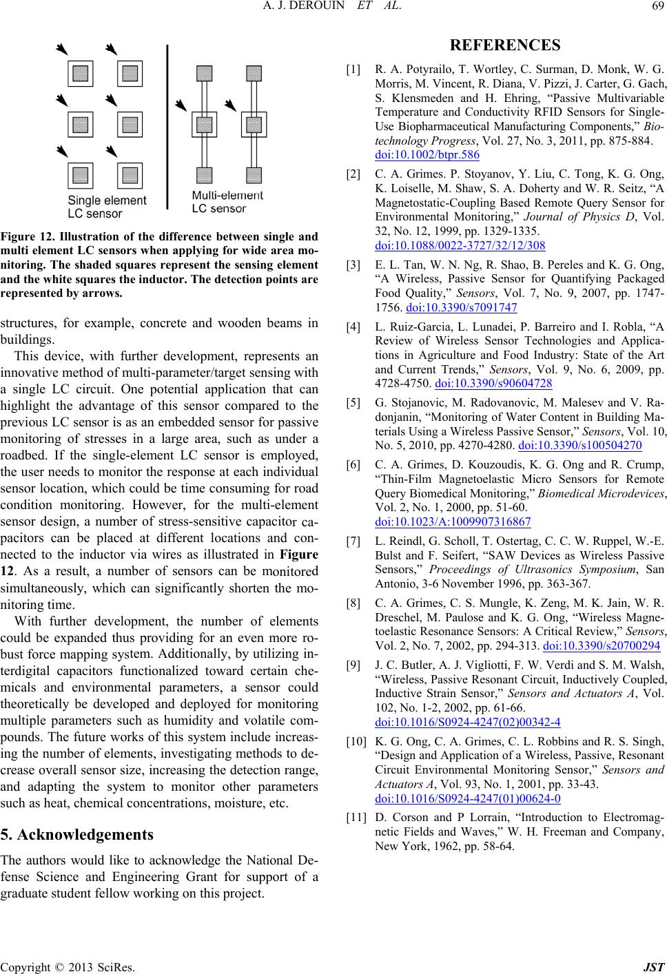

A. J. DEROUIN ET AL.

Figure 12. Illustration of the difference between single and

multi element LC sensors when applying for wide area mo-

nitoring. The shaded squares represent the sensing element

and the white squares the inductor. The detec tion points are

represented by arrows.

structures, for example, concrete and wooden beams in

buildings.

This device, with further development, represents an

innovative method of multi-parameter/target sen sing with

a single LC circuit. One potential application that can

highlight the advantage of this sensor compared t

previous LC sensor is as an embedded sensor for pas

monitoring of stresses in a large area, such as under a

roadbed. If the single-element LC sensor is employed,

the user need s to monitor the response at each individual

sensor location, which could be time consuming for road

condition monitoring. However, for the multi-element

sensor design, a number of stress-sensitive capacito

pacitors can be placed at different locations and con-

nected to the inductor via wires as illustrated in Figure

12. As a result, a number of sensors can be md

tem. Additionally, by utilizing in-

o the

sive

r ca-

onitore

simultaneously, which can significantly shorten the mo-

nitoring time.

With further development, the number of elements

could be expanded thus providing for an even more ro-

bust force mapping sys

terdigital capacitors functionalized toward certain che-

micals and environmental parameters, a sensor could

theoretically be developed and deployed for monitoring

multiple parameters such as humidity and volatile com-

pounds. The future works of this system include increas-

ing the number of elements, investigating methods to de-

crease overall sensor size, increasing the detection range,

and adapting the system to monitor other parameters

such as heat, chemical concentrations, moisture, etc.

5. Acknowledgements

The authors would like to acknowledge the National De-

fense Science and Engineering Grant for support of a

graduate studen t fellow working on this project.

REFERENCES

[1] R. A. Potyrailo, T. Wortley, C. Surman, D. Monk, W. G.

Morris, M. Vincent, R. Diana, V. Pizzi, J. Carter, G. Gach,

S. Klensmeden and H. Ehring, “Passive Multivariable

Temperature and Conductivity RFID Sensors for Single-

Use Biopharmaceutical Manufacturing Components,” Bio-

technology Progress, Vol. 27, No. 3, 2011, pp. 875-884.

doi:10.1002/btpr.586

[2] C. A. Grimes. P. Stoyanov, Y. Liu, C. Tong, K. G. Ong,

K. Loiselle, M. Shaw, S. A. Doherty and W. R. Seitz, “A

Magnetostatic-Coupling Based Remote Query Sensor for

Environmental Monitoring,” Journal of Physics D, Vol.

32, No. 12, 1999, pp. 1329-1335.

doi:10.1088/0022-3727/32/12/308

[3] E. L. Tan, W. N. Ng, R. Shao, B. Pereles and K. G. Ong,

or Quantifying Packaged

ol. 7, No. 9, 2007, pp. 1747-

“A Wireless, Passive Sensor f

Food Quality,” Sensors, V

1756. doi:10.3390/s7091747

[4] L. Ruiz-Garcia, L. Lunadei, P. Barreiro and I. Robla, “A

Review of Wireless Sensor Technologies and Applica-

tions in Agriculture and Food Industry: State of the Art

and Current Trends,” Sensors, Vol. 9, No. 6, 2009, pp.

4728-4750. doi:10.3390/s90604728

, M. Radovanovic, M. M[5] G. Stojanovicalesev and V. Ra-

donjanin, “Monitoring of Water Content in Building Ma-

terials Using a Wireless Passive Sensor,” Sensors, Vol. 10,

No. 5, 2010, pp. 4270-4280. doi:10.3390/s100504270

[6] C. A. Grimes, D. Kouzoudis, K. G. Ong and R. Crump,

“Thin-Film Magnetoelastic Micro Sensors for Remote

Query Biomedical Monitoring,” Biomedical Microdevices,

Vol. 2, No. 1, 2000, pp. 51-60.

doi:10.1023/A:1009907316867

[7] L. Reindl, G. Scholl, T. Ostertag, C. C. W. Ruppel, W.-E.

Bulst and F. Seifert, “SAW Devices as Wireless Passive

Sensors,” Proceedings of Ultrasonics Symposium, San

Antonio, 3-6 November 1996, pp. 363-367.

[8] C. A. Grimes, C. S. Mungle, K. Zeng, M. K. Jain, W. R.

Dreschel, M. Paulose and K. G. Ong, “Wireless Magne-

toelastic Resonance Sensors: A Critical Review,” Sensors,

Vol. 2, No. 7, 2002, pp. 294-313. doi:10.3390/s20700294

[9] J. C. Butler, A. J. Vigliotti, F. W. Verdi and S. M. Walsh,

“Wireless, Passive Resonant Circuit, Inductively Coupled,

Inductive Strain Sensor,” Sensors and Actuators A, Vol.

102, No. 1-2, 2002, pp. 61-66.

doi:10.1016/S0924-4247(02)00342-4

[10] K. G. Ong, C. A. Grimes, C. L. Robbins and R. S. Singh,

“Design and Application of a Wireless, Passive, Resonant

Circuit Environmental Monitoring Sensor,” Sensors and

Actuators A, Vol. 93, No. 1, 2001, pp. 33-43.

doi:10.1016/S0924-4247(01)00624-0

[11] D. Corson and P Lorrain, “Introduction to Electromag-

netic Fields and Waves,” W. H. Freeman and Company,

New York, 1962, pp. 58-64.