The Forward Exchange Rate Unbiasedness Hypothesis: A Single Break Unit Root and Cointegration Analysis

doi:10.4236/me.2013.49066

Paper Menu >>

Journal Menu >>

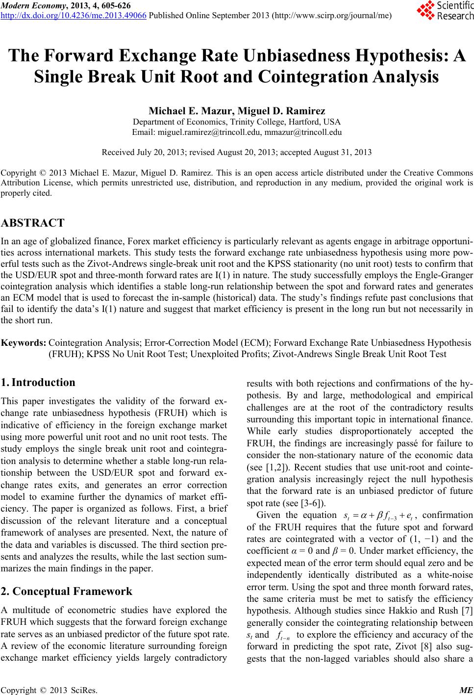Modern Economy, 2013, 4, 605-626

http://dx.doi.org/10.4236/me.2013.49066 Published Online September 2013 (http://www.scirp.org/journal/me)

The Forward Exchange Rate Unbiasedness Hypothesis: A

Single Break Unit Root and Cointegration Analysis

Michael E. Mazur, Miguel D. Ramirez

Department of Economics, Trinity College, Hartford, USA

Email: [email protected], [email protected]

Received July 20, 2013; revised August 20, 2013; accepted August 31, 2013

Attribution License, which permits unrestricted use, distribution, and reproduction in any medium, provided the original work is

properly cited.

ABSTRACT

In an age of globalized finance, Forex market efficiency is particularly relevant as agents engage in arbitrage opportuni-

ties across international markets. This study tests the forward exchange rate unbiasedness hypothesis using more pow-

erful tests such as the Zivot-Andrews single-break unit root and the KPSS stationarity (no unit root) tests to confirm that

the USD/EUR spot and three-month forward rates are I(1) in nature. The study successfully employs the Engle-Granger

cointegration analysis which identifies a stable long-run relationship between the spot and forward rates and generates

an ECM model that is used to forecast the in-sample (historical) data. The study’s findings refute past conclusions that

fail to identify the data’s I(1) nature and suggest that market efficiency is present in the long run but not necessarily in

the short run.

Keywords: Cointegration Analysis; Error-Correction Model (ECM); Forward Exchange Rate Unbiasedness Hypothesis

(FRUH); KPSS No Unit Root Test; Unexploited Profits; Zivot-Andrews Single Break Unit Root Test

1. Introduction

This paper investigates the validity of the forward ex-

change rate unbiasedness hypothesis (FRUH) which is

indicative of efficiency in the foreign exchange market

using more powerful unit root and no unit root tests. The

study employs the single break unit root and cointegra-

tion analysis to determine whether a stable long-run rela-

tionship between the USD/EUR spot and forward ex-

change rates exits, and generates an error correction

model to examine further the dynamics of market effi-

ciency. The paper is organized as follows. First, a brief

discussion of the relevant literature and a conceptual

framework of analyses are presented. Next, the nature of

the data and variables is discussed. The third section pre-

sents and analyzes the results, while the last section sum-

marizes the main findings in the paper.

2. Conceptual Framework

A multitude of econometric studies have explored the

FRUH which suggests that the forward foreign exchange

rate serves as an unbiased predictor of the future spot rate.

A review of the economic literature surrounding foreign

exchange market efficiency yields largely contradictory

results with both rejections and confirmations of the hy-

pothesis. By and large, methodological and empirical

challenges are at the root of the contradictory results

surrounding this important topic in international finance.

While early studies disproportionately accepted the

FRUH, the findings are increasingly passé for failure to

consider the non-stationary nature of the economic data

(see [1,2]). Recent studies that use unit-root and cointe-

gration analysis increasingly reject the null hypothesis

that the forward rate is an unbiased predictor of future

spot rate (see [3-6]).

Given the equation 3ttt









, confirmation

of the FRUH requires that the future spot and forward

rates are cointegrated with a vector of (1, −1) and the

coefficient α = 0 and β = 0. Under market efficiency, the

expected mean of the error term should equal zero and be

independently identically distributed as a white-noise

error term. Using the spot and three month forward rates,

the same criteria must be met to satisfy the efficiency

hypothesis. Although studies since Hakkio and Rush [7]

generally consider the cointegrating relationship between

st and tn



to explore the efficiency and accuracy of the

forward in predicting the spot rate, Zivot [8] also sug-

gests that the non-lagged variables should also share a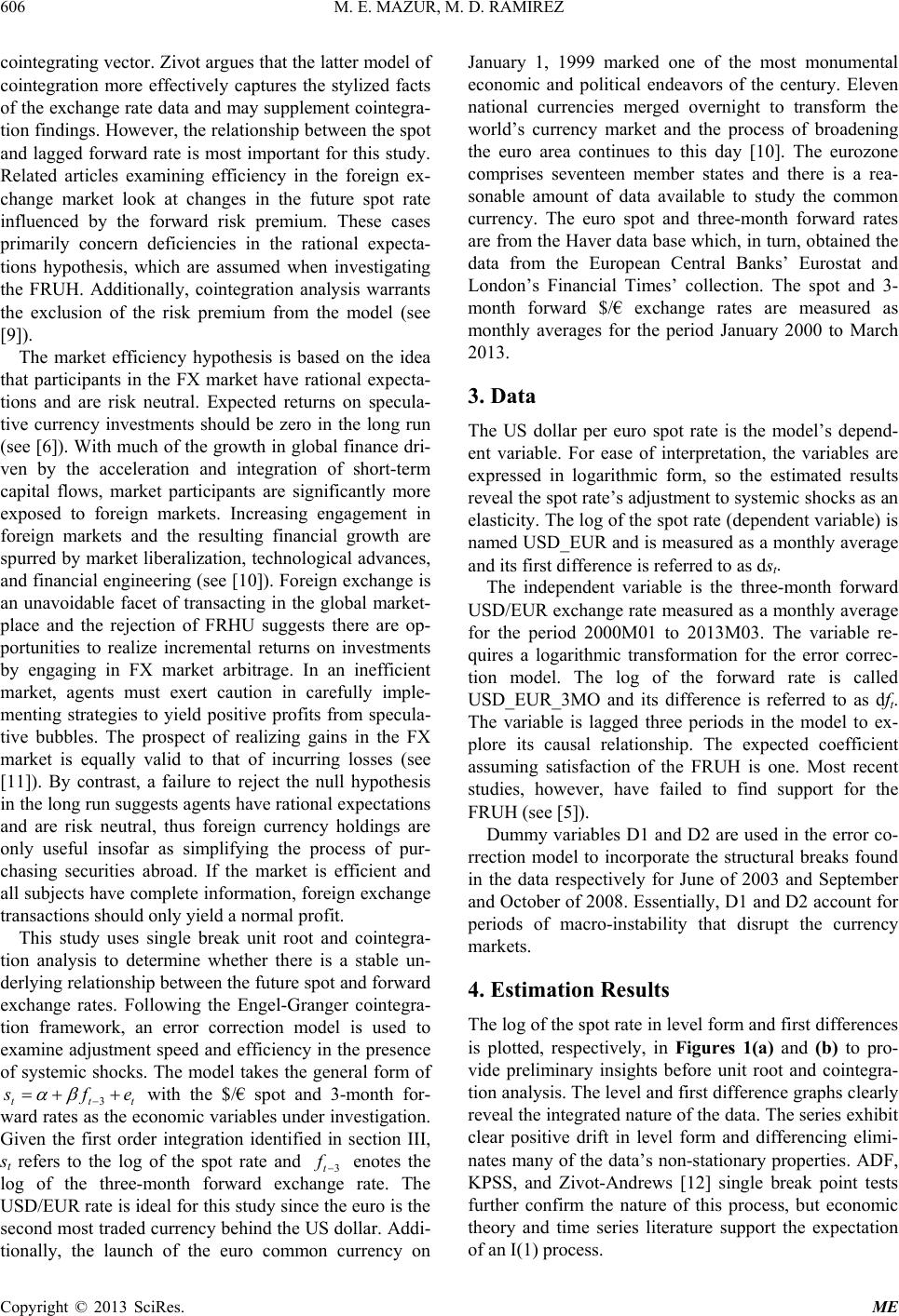

M. E. MAZUR, M. D. RAMIREZ

606

cointegrating vector. Zivot argues that the latter model of

cointegration more effectively captures the stylized facts

of the exchange rate data and may supplement cointegra-

tion findings. However, the relationship between the spot

and lagged forward rate is most important for this study.

Related articles examining efficiency in the foreign ex-

change market look at changes in the future spot rate

influenced by the forward risk premium. These cases

primarily concern deficiencies in the rational expecta-

tions hypothesis, which are assumed when investigating

the FRUH. Additionally, cointegration analysis warrants

the exclusion of the risk premium from the model (see

[9]).

The market efficiency hypothesis is based on the idea

that participants in the FX market have rational expecta-

tions and are risk neutral. Expected returns on specula-

tive currency investments should be zero in the long run

(see [6]). With much of the growth in global finance dri-

ven by the acceleration and integration of short-term

capital flows, market participants are significantly more

exposed to foreign markets. Increasing engagement in

foreign markets and the resulting financial growth are

spurred by market liberalization, technological advances,

and financial engineering (see [10]). Foreign exchange is

an unavoidable facet of transacting in the global market-

place and the rejection of FRHU suggests there are op-

portunities to realize incremental returns on investments

by engaging in FX market arbitrage. In an inefficient

market, agents must exert caution in carefully imple-

menting strategies to yield positive profits from specula-

tive bubbles. The prospect of realizing gains in the FX

market is equally valid to that of incurring losses (see

[11]). By contrast, a failure to reject the null hypothesis

in the long run suggests agents have rational expectations

and are risk neutral, thus foreign currency holdings are

only useful insofar as simplifying the process of pur-

chasing securities abroad. If the market is efficient and

all subjects have complete information, foreign exchange

transactions should only yield a normal profit.

This study uses single break unit root and cointegra-

tion analysis to determine whether there is a stable un-

derlying relationship between the future spot and forward

exchange rates. Following the Engel-Granger cointegra-

tion framework, an error correction model is used to

examine adjustment speed and efficiency in the presence

of systemic shocks. The model takes the general form of

3ttt







  with the $/€ spot and 3-month for-

ward rates as the economic variables under investigation.

Given the first order integration identified in section III,

st refers to the log of the spot rate and 3t

 enotes the

log of the three-month forward exchange rate. The

USD/EUR rate is ideal for this study since the euro is the

second most traded currency behind the US dollar. Addi-

tionally, the launch of the euro common currency on

January 1, 1999 marked one of the most monumental

economic and political endeavors of the century. Eleven

national currencies merged overnight to transform the

world’s currency market and the process of broadening

the euro area continues to this day [10]. The eurozone

comprises seventeen member states and there is a rea-

sonable amount of data available to study the common

currency. The euro spot and three-month forward rates

are from the Haver data base which, in turn, obtained the

data from the European Central Banks’ Eurostat and

London’s Financial Times’ collection. The spot and 3-

month forward $/€ exchange rates are measured as

monthly averages for the period January 2000 to March

2013.

3. Data

The US dollar per euro spot rate is the model’s depend-

ent variable. For ease of interpretation, the variables are

expressed in logarithmic form, so the estimated results

reveal the spot rate’s adjustment to systemic shocks as an

elasticity. The log of the spot rate (dependent variable) is

named USD_EUR and is measured as a monthly average

and its first difference is referred to as dst.

The independent variable is the three-month forward

USD/EUR exchange rate measured as a monthly average

for the period 2000M01 to 2013M03. The variable re-

quires a logarithmic transformation for the error correc-

tion model. The log of the forward rate is called

USD_EUR_3MO and its difference is referred to as dft.

The variable is lagged three periods in the model to ex-

plore its causal relationship. The expected coefficient

assuming satisfaction of the FRUH is one. Most recent

studies, however, have failed to find support for the

FRUH (see [5]).

Dummy variables D1 and D2 are used in the error co-

rrection model to incorporate the structural breaks found

in the data respectively for June of 2003 and September

and October of 2008. Essentially, D1 and D2 account for

periods of macro-instability that disrupt the currency

markets.

4. Estimation Results

The log of the spot rate in level form and first differences

is plotted, respectively, in Figures 1(a) and (b) to pro-

vide preliminary insights before unit root and cointegra-

tion analysis. The level and first difference graphs clearly

reveal the integrated nature of the data. The series exhibit

clear positive drift in level form and differencing elimi-

nates many of the data’s non-stationary properties. ADF,

KPSS, and Zivot-Andrews [12] single break point tests

further confirm the nature of this process, but economic

theory and time series literature support the expectation

of an I(1) process.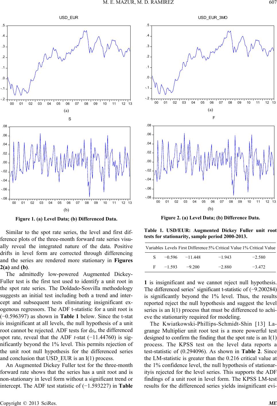

M. E. MAZUR, M. D. RAMIREZ 607

00 01 02 03 04 05 06 07 08 09 10 1112 1

US D_EUR

(a)

-.08

-.06

-.04

-.02

.00

.02

.04

.06

.08

00 01 02 03 04 05 06 07 08 09 101112 1

(b)

Figure 1. (a) Level Data; (b) Differenced Data.

Similar to the spot rate series, the level and first dif-

ference plots of the three-month forward rate series visu-

ally reveal the integrated nature of the data. Positive

drifts in level form are corrected through differencing

and the series are rendered more stationary in Figures

2(a) and (b).

The admittedly low-powered Augmented Dickey-

Fuller test is the first test used to identify a unit root in

the spot rate series. The Doldado-Sosvilla methodology

suggests an initial test including both a trend and inter-

cept and subsequent tests eliminating insignificant ex-

ogenous regressors. The ADF t-statistic for a unit root is

(−0.596397) as shown in Table 1 below. Since the t-stat

is insignificant at all levels, the null hypothesis of a unit

root cannot be rejected. ADF tests for dst, the differenced

spot rate, reveal that the ADF t-stat (−11.44760) is sig-

nificantly beyond the 1% level. This permits rejection of

the unit root null hypothesis for the differenced series

and conclusion that USD_EUR is an I(1) process.

An Augmented Dickey Fuller test for the three-month

forward rate shows that the series has a unit root and is

non-stationary in level form without a significant trend or

intercept. The ADF test statistic of (−1.593227) in Table

00 0102 03 0405 0607 0809101112 1

USD_EUR_3MO

(a)

-.08

-.06

-.04

-.02

.00

.02

.04

.06

.08

00 01 02 0304 05 06 07 08 09 10 11121

(b)

Figure 2. (a) Level Data; (b) Difference Data.

Table 1. USD/EUR: Augmented Dickey Fuller unit root

tests for stationarity, sample period 2000-2013.

VariablesLevelsFirst Difference5% Critical Value 1% Critical Value

S −0.596 −11.448 −1.943 −2.580

F −1.593 −9.200 −2.880 −3.472

1 is insignificant and we cannot reject null hypothesis.

The differenced series’ significant t-statistic of (−9.200284)

is significantly beyond the 1% level. Thus, the results

reported reject the null hypothesis and suggest the level

series is an I(1) process that must be differenced to achi-

eve the stationarity required for modeling.

The Kwiatkowski-Phillips-Schmidt-Shin [13] La-

grange Multiplier unit root test is a more powerful test

designed to confirm the finding that the spot rate is an I(1)

process. The KPSS test on the level data reports a

test-statistic of (0.294096). As shown in Table 2. Since

the LM-statistic is greater than the 0.216 critical value at

the 1% confidence level, the null hypothesis of stationar-

ityis rejected for the level series. This supports the ADF

findings of a unit root in level form. The KPSS LM-test

results for the differenced series yields insignificant evi-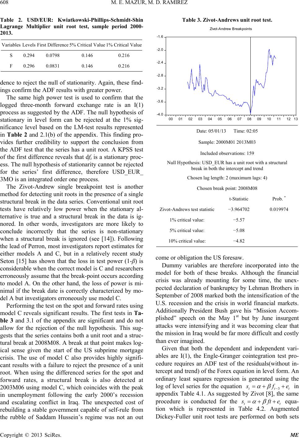

M. E. MAZUR, M. D. RAMIREZ

608

Table 2. USD/EUR: Kwiatkowski-Phillips-Schmidt-Shin

Lagrange Multiplier unit root test, sample period 2000-

2013.

Variables Levels First Difference 5% Critical Value 1% Critical Value

S 0.294 0.0798 0.146 0.216

F 0.296 0.0831 0.146 0.216

dence to reject the null of stationarity. Again, these find-

ings confirm the ADF results with greater power.

The same high power test is used to confirm that the

logged three-month forward exchange rate is an I(1)

process as suggested by the ADF. The null hypothesis of

stationary in level form can be rejected at the 1% sig-

nificance level based on the LM-test results represented

in Table 2 and 2.1(b) of the appendix. This finding pro-

vides further credibility to support the conclusion from

the ADF test that the series has a unit root. A KPSS test

of the first difference reveals that dft is a stationary proc-

ess. The null hypothesis of stationarity cannot be rejected

for the series’ first difference, therefore USD_EUR_

3MO is an integrated order one process.

The Zivot-Andrew single breakpoint test is another

method for detecting unit roots in the presence of a single

structural break in the data series. Conventional unit root

tests have relatively low power when the stationary al-

ternative is true and a structural break in the data is ig-

nored. In other words, investigators are more likely to

conclude incorrectly that the series is non-stationary

when a structural break is ignored (see [14]). Following

the lead of Perron, most investigators report estimates for

either models A and C, but in a relatively recent study

Seton [15] has shown that the loss in test power (1-β) is

considerable when the correct model is C and researchers

erroneously assume that the break-point occurs according

to model A. On the other hand, the loss of power is mi-

nimal if the break date is correctly characterized by mo-

del A but investigators erroneously use model C.

Performing the test on the spot and forward rates using

model C reveals significant results. The first tests in Ta-

ble 3 and 3.1 of the appendix are significant and do not

allow for the rejection of the null hypothesis. This sug-

gests that the series contains both a unit root and a struc-

tural break at 2008M08. A break at that point makes log-

ical sense given the start of the US subprime mortgage

crisis. The use of model C also provides highly signifi-

cant results with a failure to reject the presence of a unit

root. When using the differenced series for the spot and

forward rates, a structural break is also detected at

2003M06 using model C, which coincides with the peak

in unemployment following the early 2000’s recession

and escalating conflict in Iraq. The unexpected cost of

rebuilding a stable government capable of self-rule from

the rubble of Saddam Hussein’s regime was not an out

Table 3. Zivot-Andrews unit root test.

-4.0

-3.6

-3.2

-2.8

-2.4

-2.0

-1.6

00 01 02 03 04 05 0607 08 09 10 11 121

Zivot-A ndrew Breakp oint s

Date: 05/01/13 Time: 02:05

Sample: 2000M01 2013M03

Included observations: 159

Null Hypothesis: USD_EUR has a unit root with a structural

break in both the intercept and trend

Chosen lag length: 2 (maximum lags: 4)

Chosen break point: 2008M08

t-Statistic Prob.

Zivot-Andrews test statistic −3.964702 0.019974

1% critical value: −5.57

5% critical value: −5.08

10% critical value: −4.82

come or obligation the US foresaw.

Dummy variables are therefore incorporated into the

model for both of these breaks. Although the financial

crisis was already mounting for some time, the unex-

pected declaration of bankruptcy by Lehman Brothers in

September of 2008 marked both the intensification of the

U.S. recession and the crisis in world financial markets.

Additionally President Bush gave his “Mission Accom-

plished” speech on the May 1st but by June insurgent

attacks were intensifying and it was becoming clear that

the mission in Iraq would be far more difficult and costly

than ever imagined.

Given that both the dependent and independent vari-

ables are I(1), the Engle-Granger cointegration test pro-

cedure requires an ADF test of the residuals(without in-

tercept and trend) of the Forex equation in level form. An

ordinary least squares regression is generated using the

log of level series for the equation 3ttt







  in

appendix Table 4.1. As suggested by Zivot [8], the same

procedure is conducted for the tt

ft e





  equa-

tion which is represented in Table 4.2. Augmented

Dickey-Fuller unit root tests are performed on both sets

M. E. MAZUR, M. D. RAMIREZ 609

of residuals in Tables 4.1(b) and 4.2(b) of the appendix.

The results for the residuals including the lagged term

overwhelmingly support the rejection of the null hy-

pothesis of a unit root for all significance levels. The test

in simple form is less significant but the t-statistics are

still strong enough to reject the null of a unit root at the

5% level of significance. The stationary nature of the

residuals in level form suggests that st is cointegrated

with both 3t

 and

. The identification of a cointe-

grating vector is important in that it identifies a stable

long-run relationship that keeps the variables in propor-

tion over time, and suggests that the market is efficient in

the long run. Following the Engle-Granger representation

theorem, an error correction model that includes the re-

siduals is generated to reconcile the short and long-run

behavior of the underlying relationship between the for-

ward and spot exchange rates.

The final model shown in Model 1 is significant and

with a high degree of explanatory and forecasting power.

The error correction model incorporates the forward va-

able, error correction term, and two dummy variables:

D1 for 2003M06 and D2 for 2008M09-M10 described

above. The HAC Newey-West [16] procedure was util-

ed in estimating the ECM, thus correcting the OLS stan-

rd errors for both autocorrelation and heteroscedasticity.

The Durbin Watson test statistic is 2.1 and suggests that

the final model does not suffer from first order serial

correlation. All of the terms except for the constant gen-

Model 1. USD/EUR: Error Correction Model; dependent

variable is: (S), 2000-2013.

OLS Regressions

Variable Coefficient Std. Error t-Statistic Prob.

C 5.87E-05 6.93E-05 0.846956 0.3984

F 1.001182 0.003877 258.2166 0.0000

EC1(−1) −0.046752 0.021973 −2.127676 0.0350

D1 −0.001047 0.000250 −4.182255 0.0000

D2 −0.001122 0.000310 −3.619541 0.0004

AR(1) −0.288958 0.092038 −3.139549 0.0020

R-squared 0.998 Mean dependent var 0.002

Adjusted R-squared 0.998 S.D. dependent var 0.025

S.E. of regression 0.001 Akaike info criterion −10.611

Sum squared resid 0.000 Schwarz criterion −10.495

Log likelihood 838.994 Hannan-Quinn criter. −10.564

F-statistic 14495.59 Durbin-Watson stat 2.100

Prob(F-statistic) 0.000

ate high t-statistics and are significant at the 5% signi-

ficance level. The EC1(−1) term is significant at the 5%

level and suggests that a deviation of 10 percent from the

long run equilibrium during the current period is cor-

rected in the subsequent period by approximately 0.5

percent. The addition of the D2 term, given that its inclu-

sion makes theoretical sense, increases the Adjusted R

squared and enhances the degree of accuracy for the final

model.

The fact that the constant is not significantly different

from zero supports the efficiency hypothesis.

The estimated coefficient for the forward rate is

1.001182 with a t-stat of 258.2166. This result is highly

significant and since it is close to 1, the model fulfills the

FRUH criteria. The failure to reject the null hypothesis

serves to support the use of the forward rate as an unbi-

ased estimator of the future spot rate. The evidence for

the dollar-euro rate suggests support for market effi-

ciency in the long run but not necessarily in the short run

because a disequilibrium exists between the two vari-

ables, suggesting that expected returns to speculators are

not zero in the short run (see [7]). In general, the results

suggest that participants in the foreign exchange market

are risk neutral and have little to gain from speculation in

the long run.

EC models were also used to track the historical data

on the percentage change in the spot rate for the period

under review. Figure 3 below shows that the model was

able to track the turning points in the actual series quite

well. s refers to the actual series and (sf) denotes the

in-sample forecast. In addition, Figure 4 below shows

that the Theil inequality coefficient for this model is

0.02270, which is well below the threshold value of 0.3,

and suggests that the predictive power of the model is

quite good (see [17]). The Theil coefficients can be de-

composed into three major components: the bias, vari-

ance, and covariance terms. Ideally, the bias and variance

components should equal zero, while the covariance

-.08

-.06

-.04

-.02

.00

.02

.04

.06

.08

00 01 02 03 04 05 0607 0809 101112 13

S: ActualSF: In- Sample Forecast

Figure 3. Actual and simulated percentage changes in the

spot rate.

M. E. MAZUR, M. D. RAMIREZ

610

Figure 4. Theil inequality coefficient for in-sample forecast.

proportion should equal one. The reported estimates su-

ggest that all of these ratios are close to their optimum

values (bias = 0.0000, variance = 0.0067, and covariance

= 0.9932). Sensitivity analysis on the coefficients also

revealed that changes in the initial or ending period did

not alter the predictive power of the selected models (re-

sults are available upon request).

5. Conclusion

Efficiency in the foreign exchange market is especially

relevant in the world of globalized finance since market

agents are frequently and increasingly transacting both at

home and abroad. This study shows that the spot and

three-month forward exchange rates are I(1) processes

using the more powerful KPPS stationarity test and the

Zivot Andrews single break unit root test. Following the

Engle-Granger cointegration analysis framework, a long-

run stable relationship between the three-month forward

exchange rate and the future spot rate is identified which

suggests that the forward rate contains useful information

about the spot rate; in other words, it supports market

efficiency in the long run. Insofar as the error correction

model is concerned, it provided further support for the

forward exchange rate unbiasedness hypothesis. With a

high degree of power, the results of the model fulfill the

final two criteria for market efficiency, viz., a constant

equal to 0 and a coefficient of 1. However, the results

also suggest that there is a disequilibrium in the short run

that is only partially corrected in subsequent periods,

suggesting that, in the short run, there might be unex-

ploited profit opportunities for speculators and/or a time-

varying risk premium. Needless to say, economists have

debated the issue of exchange market efficiency since the

70’s and this study, although supportive of market effi-

ciency in the long run, will by no means settle the con-

troversy. Finally, the endogenously determined structural

breaks in the data indicate that, since the common cur-

rency’s inception, volatility and disruption of the Forex

market have been generated by both the un-expected

costs associated with the war in Iraq and the 2008 global

financial crisis.

REFERENCES

[1] R. M. Levich, “Empirical Studies of Exchange Rates,

Price Behavior, Rate Determination, and Market Effi-

ciency,” In: R. W. Jones and P. B. Kennen, Eds., Hand-

book of International Economics, Vol. II, Elsevier, Am-

sterdam, 1978, pp. 979-1040.

[2] J. A. Frenkel, “Flexible Exchange Rates, Prices, and the

Role of News: Lessons from the 1970s,” In: R. A. Bat-

chelor and G. E. Wood, Eds., Exchange Rate Policy, Ma-

cmillan, London, 1982.

[3] R. E. Cumby and M. Obstfeld, “International Interest

Rate and Price Level Linkages under Flexible Exchange

Rates: A Review of the Evidence,” 1984.

[4] C. Engel, “The Forward Discount Anomaly and the Risk

Premium: A Survey of Recent Evidence,” Journal of Em-

pirical Finance, Vol. 3, No. 2, 1996, pp. 123-192.

[5] J. Olmo and K. Pilbeam, “Uncovered Interest Parity and

the Efficiency of the Foreign Exchange Market: A Re-

examination of the Evidence,” International Journal of

Finance and Economics, Vol. 16, No. 2, 2011, pp. 189-

204. doi:10.1002/ijfe.429

[6] V. Ukpolo, “Exchange Rate Market Efficiency; Further

Evidence from Cointegration Tests,” Applied Economics

Letters, Vol. 2, No. 6, 1995, pp. 196-198.

doi:10.1080/135048595357438

[7] C. S. Hakkio and M. Rush, “Cointegration: How Short Is

the Long Run?” Journal of International Money and Fi-

nance, Vol. 10, No. 4, 1991, pp. 571-581.

doi:10.1016/0261-5606(91)90008-8

[8] E. Zivot, “Cointegration and Forward and Spot Exchange

Rate Regressions,” 1998.

http://128.118.178.162/eps/em/papers/9812/9812001.pdf

[9] M. Kuhl, “Cointegration in the Foreign Exchange Market

and Market Efficiency since the Introduction of the Euro:

Evidence Based on bivariate Cointegration Analyses,”

2007.

[10] D. W. Duisenberg, “Recent Developments and Trends in

World Financial Market,” 2000.

http://www.ecb.int/press/key/date/2000/html/sp001114.en

.html

[11] A. C. Jung and V. Wieland, “Forward Rates and Spot

Rates in the European Monetary System-Forward Market

Efficiency,” Weltwirtschaftliches Archiv, Vol. 126, No. 4,

1990, pp. 615-629. doi:10.1007/BF02707471

[12] E. Zivot and D. Andrews, “Further Evidence of Great

Crash, the Oil Price Shock, and Unit Root Hypothesis,”

Journal of Business and Economic Statistics, Vol. 10, No.

3, 1992, pp. 251-270.

doi:10.1080/07350015.1992.10509904

[13] D. Kwaitkowski, P. C. B. Phillips, P. Schmidt and Y.

Shin, “Testing the Null Hypothesis of Stationarity against

the Alternative of a Unit Root,” Journal of Econometrics,

Vol. 54, No. 1-3, 1992, pp. 159-178.

doi:10.1016/0304-4076(92)90104-Y

[14] P. Perron, “The Great Crash, the Oil Price Shock and the

Unit Root Hypothesis,” Econometrica, Vol. 57, No. 6,

1989, pp. 1361-1401. doi:10.2307/1913712

[15] A. Seton, “On Unit Root Tests when the Alternative Is a

M. E. MAZUR, M. D. RAMIREZ

611

Trend Break Stationary Process,” Journal Of Business

and Economic Statistics, Vol. 21, No. 1, 2003, pp. 174-

184. doi:10.1198/073500102288618874

[16] W. K. Newey and K. West, “A Simple Positive Semi-

Definite Heteroscedasticity and Autocorrelation Consis-

tent Covariance Matrix,” Econometrica, Vol. 55, No. 3,

1987, pp. 703-708. doi:10.2307/1913610

[17] H. Theil, “Applied Economic Forecasting,” North-Holland,

Amsterdam, 1966.

M. E. MAZUR, M. D. RAMIREZ

612

Appendix:

ADF Tests: Table 1.1.

Null Hypothesis: USD_EUR has a unit root

Exogenous: Constant, Linear Trend

Lag Length: 1 (Automatic-based on SIC, maxlag = 13)

t-Statistic Prob.*

Augmented Dickey-Fuller test statistic −1.879977 0.6602

Test critical values: 1% level −4.017568

5% level −3.438700

10% level −3.143666

*MacKinnon (1996) one-sided p-values.

Augmented Dickey-Fuller Test Equation

Dependent Variable: D(USD_EUR)

Method: Least Squares

Date: 04/30/13 Time: 23:55

Sample (adjusted): 2000M03 2013M03

Included observations: 157 after adjustments

Variable Coefficient Std. Error t-Statistic Prob.

USD_EUR (−1) −0.037629 0.020016 −1.879977 0.0620

D(USD_EUR (−1)) 0.322964 0.076939 4.197673 0.0000

C 0.001599 0.004044 0.395337 0.6931

@TREND(2000M01 8.38E − 05 7.31E − 05 1.146264 0.2535

R-squared 0.114862 Mean dependent var 0.001760

Adjusted R-squared 0.097506 S.D. dependent var 0.025432

S.E. of regression 0.024161 Akaike info criterion −4.583039

Sum squared resid 0.089311 Schwarz criterion −4.505172

Log likelihood 363.7685 Hannan-Quinn criter. −4.551414

F-statistic 6.618140 Durbin-Watson stat 1.906269

Prob (F-statistic) 0.000311

Table 1.2.

Null Hypothesis: USD_EUR has a unit root

Exogenous: Constant

Lag Length: 1 (Automatic-based on SIC, maxlag = 13)

t-Statistic Prob.*

Augmented Dickey-Fuller test statistic −1.627012 0.4664

Test critical values: 1% level −3.472259

5% level −2.879846

10% level −2.576610

M. E. MAZUR, M. D. RAMIREZ 613

Continued

*MacKinnon (1996) one-sided p-values.

Augmented Dickey-Fuller Test Equation

Dependent Variable: D(USD_EUR)

Method: Least Squares

Date: 05/01/13 Time: 00:03

Sample (adjusted): 2000M03 2013M03

Included observations: 157 after adjustments

Variable Coefficient Std. Error t-Statistic Prob.

USD_EUR (−1) −0.018971 0.011660 −1.627012 0.1058

D(USD_EUR (−1)) 0.310732 0.076273 4.073951 0.0001

C 0.004800 0.002927 1.640082 0.1030

R-squared 0.107261 Mean dependent var 0.001760

Adjusted R-squared 0.095667 S.D. dependent var 0.025432

S.E. of regression 0.024185 Akaike info criterion −4.587226

Sum squared resid 0.090078 Schwarz criterion −4.528827

Log likelihood 363.0973 Hannan-Quinn criter. −4.563508

F-statistic 9.251392 Durbin-Watson stat 1.906204

Prob (F-statistic) 0.000161

Table 1.3.

Null Hypothesis: USD_EUR has a unit root

Exogenous: None

Lag Length: 1 (Automatic-based on SIC, maxlag = 13)

t-Statistic Prob.*

Augmented Dickey-Fuller test statistic −0.596397 0.4576

Test critical values: 1% level −2.579774

5% level −1.942869

10% level −1.615359

*MacKinnon (1996) one-sided p-values.

Augmented Dickey-Fuller Test Equation

Dependent Variable: D(USD_EUR)

Method: Least Squares

Date: 04/30/13 Time: 23:56

Sample (adjusted): 2000M03 2013M03

Included observations: 157 after adjustments

Variable Coefficient Std. Error t-Statistic Prob.

USD_EUR (−1) -0.004622 0.007750 −0.596397 0.5518

D(USD_EUR (−1)) 0.310701 0.076687 4.051526 0.0001

M. E. MAZUR, M. D. RAMIREZ

614

Continued

R-squared 0.091668 Mean dependent var 0.001760

Adjusted R-squared 0.085807 S.D. dependent var 0.025432

S.E. of regression 0.024317 Akaike info criterion −4.582649

Sum squared resid 0.091652 Schwarz criterion −4.543716

Log likelihood 361.7380 Hannan-Quinn criter. −4.566837

Durbin-Watson stat 1.901715

Table 1.4.

Null Hypothesis: S has a unit root

Exogenous: Constant, Linear Trend

Lag Length: 0 (Automatic-based on SIC, maxlag = 13)

t-Statistic Prob.*

Augmented Dickey-Fuller test statistic −9.104497 0.0000

Test critical values: 1% level −4.017568

5% level −3.438700

10% level −3.143666

*MacKinnon (1996) one-sided p-values.

Augmented Dickey-Fuller Test Equation

Dependent Variable: D(S)

Method: Least Squares

Date: 05/01/13 Time: 00:19

Sample (adjusted): 2000M03 2013M03

Included observations: 157 after adjustments

Variable Coefficient Std. Error t-Statistic Prob.

S (−1) −0.698449 0.076715 −9.104497 0.0000

C 0.003469 0.003952 0.877802 0.3814

@TREND(2000M01) −2.80E − 05 4.29E − 05 −0.652052 0.5153

R-squared 0.350275 Mean dependent var 2.12E-06

Adjusted R-squared 0.341837 S.D. dependent var 0.030025

S.E. of regression 0.024359 Akaike info criterion −4.572940

Sum squared resid 0.091375 Schwarz criterion −4.514540

Log likelihood 361.9758 Hannan-Quinn criter. −4.549222

F-statistic 41.51164 Durbin-Watson stat 1.901343

Prob (F-statistic) 0.000000

M. E. MAZUR, M. D. RAMIREZ 615

Table 1.5.

Null Hypothesis: D(S) has a unit root

Exogenous: Constant

Lag Length: 2 (Automatic-based on SIC, maxlag = 13)

t-Statistic Prob.*

Augmented Dickey-Fuller test statistic −11.41115 0.0000

Test critical values: 1% level −3.473096

5% level −2.880211

10% level −2.576805

*MacKinnon (1996) one-sided p-values.

Augmented Dickey-Fuller Test Equation

Dependent Variable: D(S,2)

Method: Least Squares

Date: 05/01/13 Time: 00:30

Sample (adjusted): 2000M06 2013M03

Included observations: 154 after adjustments

Variable Coefficient Std. Error t-Statistic Prob.

D (S(−1)) −2.059546 0.180485 −11.41115 0.0000

D (S(−1),2) 0.647650 0.130722 4.954415 0.0000

D (S(−2),2) 0.214490 0.080233 2.673330 0.0083

C 0.000320 0.002176 0.147022 0.8833

R-squared 0.685197 Mean dependent var −5.97E-05

Adjusted R-squared 0.678901 S.D. dependent var 0.047635

S.E. of regression 0.026993 Akaike info criterion −4.360876

Sum squared resid 0.109290 Schwarz criterion −4.281994

Log likelihood 339.7874 Hannan-Quinn criter. −4.328834

F-statistic 108.8297 Durbin-Watson stat 1.958890

Prob (F-statistic) 0.000000

Table 1.6.

Null Hypothesis: D(S) has a unit root

Exogenous: None

Lag Length: 2 (Automatic-based on SIC, maxlag = 13)

t-Statistic Prob.*

Augmented Dickey-Fuller test statistic −11.44760 0.0000

Test critical values: 1% level −2.580065

5% level −1.942910

10% level −1.615334

M. E. MAZUR, M. D. RAMIREZ

616

Continued

*MacKinnon (1996) one-sided p-values.

Augmented Dickey-Fuller Test Equation

Dependent Variable: D(S,2)

Method: Least Squares

Date: 05/01/13 Time: 00:31

Sample (adjusted): 2000M06 2013M03

Included observations: 154 after adjustments

Variable Coefficient Std. Error t-Statistic Prob.

D (S(−1)) −2.059028 0.179865 −11.44760 0.0000

D (S(−1),2) 0.647283 0.130274 4.968635 0.0000

D (S(−2),2) 0.214285 0.079961 2.679881 0.0082

R-squared 0.685152 Mean dependent var −5.97E − 05

Adjusted R-squared 0.680982 S.D. dependent var 0.047635

S.E. of regression 0.026905 Akaike info criterion −4.373718

Sum squared resid 0.109306 Schwarz criterion −4.314557

Log likelihood 339.7763 Hannan-Quinn criter. −4.349687

Durbin-Watson stat 1.958836

Table 1.1(b)

Null Hypothesis: USD_EUR_3MO has a unit root

Exogenous: Constant, Linear Trend

Lag Length: 1 (Automatic-based on SIC, maxlag = 13)

t-Statistic Prob.*

Augmented Dickey-Fuller test statistic −1.853265 0.6738

Test critical values: 1% level −4.017568

5% level −3.438700

10% level −3.143666

*MacKinnon (1996) one-sided p-values.

Augmented Dickey-Fuller Test Equation

Dependent Variable: D(USD_EUR_3MO)

Method: Least Squares

Date: 05/01/13 Time: 01:15

Sample (adjusted): 2000M03 2013M03

Included observations: 157 after adjustments

Variable Coefficien Std. Error t-Statistic Prob.

USD_EUR_3MO(−1) −0.037143 0.020042 −1.853265 0.0658

D(USD_EUR_3MO(−1)) 0.312895 0.077209 4.052590 0.0001

C 0.001563 0.004049 0.385970 0.7001

M. E. MAZUR, M. D. RAMIREZ 617

Continued

@TREND(2000M01) 8.32E − 05 7.32E − 05 1.136803 0.2574

R-squared 0.108380 Mean dependent var 0.001721

Adjusted R-squared 0.090898 S.D. dependent var 0.025400

S.E. of regression 0.024218 Akaike info criterion −4.578301

Sum squared resid 0.089736 Schwarz criterion −4.500435

Log likelihood 363.3967 Hannan-Quinn criter. −4.546677

F-statistic 6.199278 Durbin-Watson stat 1.907224

Prob (F-statistic) 0.000530

Table 1.2(b)

Null Hypothesis: USD_EUR_3MO has a unit root

Exogenous: Constant

Lag Length: 1 (Automatic-based on SIC, maxlag = 13)

t-Statistic Prob.*

Augmented Dickey-Fuller test statistic −1.593227 0.4837

Test critical values: 1% level −3.472259

5% level −2.879846

10% level −2.576610

*MacKinnon (1996) one-sided p-values.

Augmented Dickey-Fuller Test Equation

Dependent Variable: D(USD_EUR_3MO)

Method: Least Squares

Date: 05/01/13 Time: 01:16

Sample (adjusted): 2000M03 2013M03

Included observations: 157 after adjustments

Variable Coefficient Std. Error t-Statistic Prob.

USD_EUR_3MO(−1) −0.018630 0.011693 −1.593227 0.1132

D(USD_EUR_3MO(−1)) 0.300906 0.076558 3.930450 0.0001

C 0.004733 0.002938 1.610995 0.1092

R-squared 0.100849 Mean dependent var 0.001721

Adjusted R-squared 0.089172 S.D. dependent var 0.025400

S.E. of regression 0.024241 Akaike info criterion −4.582629

Sum squared resid 0.090494 Schwarz criterion −4.524229

Log likelihood 362.7364 Hannan-Quinn criter. −4.558911

F-statistic 8.636363 Durbin-Watson stat 1.907614

Prob(F-statistic) 0.000279

M. E. MAZUR, M. D. RAMIREZ

618

Table 1.3(b)

Null Hypothesis: USD_EUR_3MO has a unit root

Exogenous: Constant

Lag Length: 1 (Automatic-based on SIC, maxlag = 13)

t-Statistic Prob.*

Augmented Dickey-Fuller test statistic −1.593227 0.4837

Test critical values: 1% level −3.472259

5% level −2.879846

10% level −2.576610

*MacKinnon (1996) one-sided p-values.

Augmented Dickey-Fuller Test Equation

Dependent Variable: D(USD_EUR_3MO)

Method: Least Squares

Date: 05/01/13 Time: 01:16

Sample (adjusted): 2000M03 2013M03

Included observations: 157 after adjustments

Variable Coefficient Std. Error t-Statistic Prob.

USD_EUR_3MO(-1) −0.018630 0.011693 −1.593227 0.1132

D(USD_EUR_3MO(-1)) 0.300906 0.076558 3.930450 0.0001

C 0.004733 0.002938 1.610995 0.1092

R-squared 0.100849 Mean dependent var 0.001721

Adjusted R-squared 0.089172 S.D. dependent var 0.025400

S.E. of regression 0.024241 Akaike info criterion −4.582629

Sum squared resid 0.090494 Schwarz criterion −4.524229

Log likelihood 362.7364 Hannan-Quinn criter. −4.558911

F-statistic 8.636363 Durbin-Watson stat 1.907614

Prob (F-statistic) 0.000279

Table 1.4(b)

Null Hypothesis: F has a unit root

Exogenous: Constant, Linear Trend

Lag Length: 0 (Automatic-based on SIC, maxlag = 13)

t-Statistic Prob.*

Augmented Dickey-Fuller test statistic −9.200100 0.0000

Test critical values: 1% level −4.017568

5% level −3.438700

10% level −3.143666

*MacKinnon (1996) one-sided p-values.

Augmented Dickey-Fuller Test Equation

M. E. MAZUR, M. D. RAMIREZ 619

Continued

Dependent Variable: D(F)

Method: Least Squares

Date: 05/01/13 Time: 01:24

Sample (adjusted): 2000M03 2013M03

Included observations: 157 after adjustments

Variable Coefficient Std. Error t-Statistic Prob.

F(-1) −0.708141 0.076971 −9.200100 0.0000

C 0.003380 0.003959 0.853816 0.3945

@TREND(2000M01) −2.70E − 05 4.30E − 05 −0.628238 0.5308

R-squared 0.355022 Mean dependent var 6.96E-07

Adjusted R-squared 0.346645 S.D. dependent var 0.030197

S.E. of regression 0.024409 Akaike info criterion −4.568840

Sum squared resid 0.091750 Schwarz criterion −4.510441

Log likelihood 361.6539 Hannan-Quinn criter. −4.545122

F-statistic 42.38388 Durbin-Watson stat 1.903271

Prob (F-statistic) 0.000000

Table 1.5(b)

Null Hypothesis: F has a unit root

Exogenous: Constant

Lag Length: 0 (Automatic-based on SIC, maxlag = 13)

t-Statistic Prob.*

Augmented Dickey-Fuller test statistic −9.203471 0.0000

Test critical values: 1% level −3.472259

5% level −2.879846

10% level −2.576610

*MacKinnon (1996) one-sided p-values.

Augmented Dickey-Fuller Test Equation

Dependent Variable: D(F)

Method: Least Squares

Date: 05/01/13 Time: 01:27

Sample (adjusted): 2000M03 2013M03

Included observations: 157 after adjustments

Variable Coefficient Std. Error t-Statistic Prob.

F(−1) −0.706704 0.076787 −9.203471 0.0000

C 0.001217 0.001949 0.624309 0.5333

R-squared 0.353369 Mean dependent var 6.96E-07

Adjusted R-squared 0.349197 S.D. dependent var 0.030197

S.E. of regression 0.024361 Akaike info criterion −4.579019

Sum squared resid 0.091985 Schwarz criterion −4.540086

Log likelihood 361.4530 Hannan-Quinn criter. −4.563207

F-statistic 84.70387 Durbin-Watson stat 1.900803

Prob (F-statistic) 0.000000

M. E. MAZUR, M. D. RAMIREZ

620

Table 1.6(b)

Null Hypothesis: F has a unit root

Exogenous: None

Lag Length: 0 (Automatic-based on SIC, maxlag = 13)

t-Statistic Prob.*

Augmented Dickey-Fuller test statistic −9.200284 0.0000

Test critical values: 1% level −2.579774

5% level −1.942869

10% level −1.615359

*MacKinnon (1996) one-sided p-values.

Augmented Dickey-Fuller Test Equation

Dependent Variable: D(F)

Method: Least Squares

Date: 05/01/13 Time: 01:28

Sample (adjusted): 2000M03 2013M03

Included observations: 157 after adjustments

Variable Coefficient Std. Error t-Statistic Prob.

F(−1) −0.703454 0.076460 −9.200284 0.0000

R-squared 0.351743 Mean dependent var 6.96E − 07

Adjusted R-squared 0.351743 S.D. dependent var 0.030197

S.E. of regression 0.024313 Akaike info criterion −4.589247

Sum squared resid 0.092216 Schwarz criterion −4.569780

Log likelihood 361.2559 Hannan-Quinn criter. −4.581341

Durbin-Watson stat 1.901439

KPSS tests: Table 2.1.

Null Hypothesis: USD_EUR is stationary

Exogenous: Constant, Linear Trend

Bandwidth: 10 (Newey-West automatic) using Bartlett kernel

LM-Stat.

Kwiatkowski-Phillips-Schmidt-Shin test statistic 0.294096

Asymptotic critical values*: 1% level 0.216000

5% level 0.146000

10% level 0.119000

*Kwiatkowski-Phillips-Schmidt-Shin (1992, Table 1)

Residual variance (no correction) 0.009552

HAC corrected variance (Bartlett kernel) 0.085235

KPSS Test Equation

M. E. MAZUR, M. D. RAMIREZ 621

Continued

Dependent Variable: USD_EUR

Method: Least Squares

Date: 05/01/13 Time: 01:33

Sample: 2000M01 2013M03

Included observations: 159

Variable Coefficient Std. Error t-Statistic Prob.

C −0.041448 0.015527 −2.669403 0.0084

@TREND(2000M01) 0.002909 0.000170 17.11939 0.0000

R-squared 0.651168 Mean dependent var 0.188391

Adjusted R-squared 0.648946 S.D. dependent var 0.166004

S.E. of regression 0.098357 Akaike info criterion −1.787927

Sum squared resid 1.518834 Schwarz criterion −1.749324

Log likelihood 144.1402 Hannan-Quinn criter. −1.772251

F-statistic 293.0734 Durbin-Watson stat 0.067298

Prob (F-statistic) 0.000000

Table 2.2.

Null Hypothesis: S is stationary

Exogenous: Constant, Linear Trend

Bandwidth: 1 (Newey-West automatic) using Bartlett kernel

LM-Stat.

Kwiatkowski-Phillips-Schmidt-Shin test statistic 0.079840

Asymptotic critical values*: 1% level 0.216000

5% level 0.146000

10% level 0.119000

*Kwiatkowski-Phillips-Schmidt-Shin (1992, Table 1)

Residual variance (no correction) 0.000644

HAC corrected variance (Bartlett kernel) 0.000836

KPSS Test Equation

Dependent Variable: S

Method: Least Squares

Date: 05/01/13 Time: 01:51

Sample (adjusted): 2000M02 2013M03

Included observations: 158 after adjustments

Variable Coefficient Std. Error t-Statistic Prob.

C 0.003549 0.004082 0.869288 0.3860

@TREND(2000M01) −2.51E-05 4.45E-05 −0.562515 0.5746

R-squared 0.002024 Mean dependent var 0.001557

Adjusted R-squared −0.004373 S.D. dependent var 0.025480

S.E. of regression 0.025535 Akaike info criterion −4.484941

Sum squared resid 0.101719 Schwarz criterion −4.446174

Log likelihood 356.3103 Hannan-Quinn criter. −4.469197

F-statistic 0.316423 Durbin-Watson stat 1.382589

Prob (F-statistic) 0.574573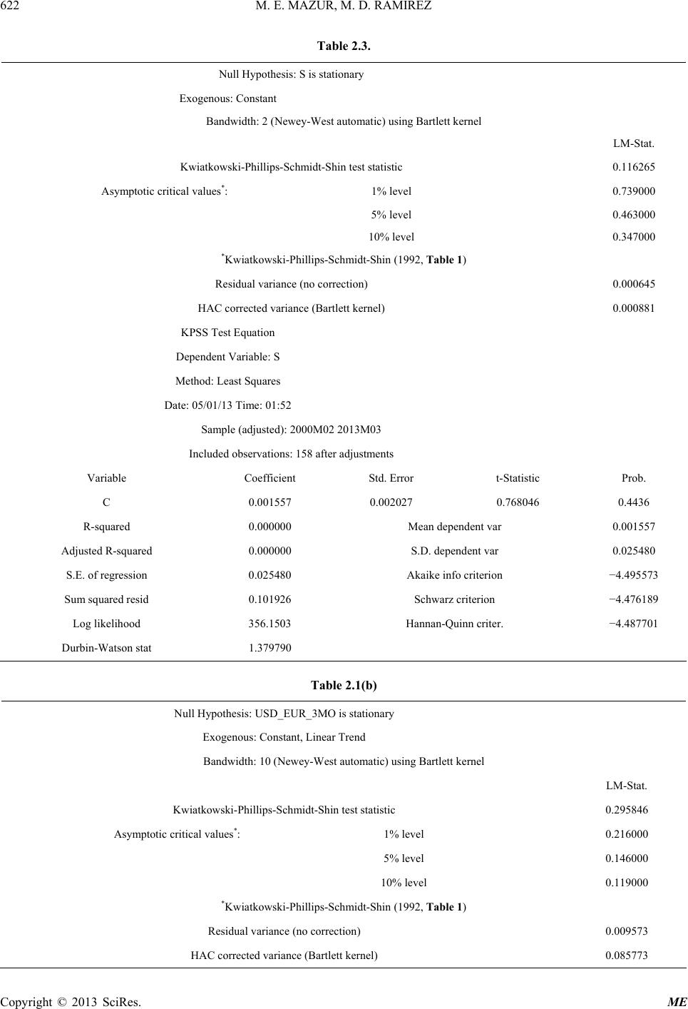

M. E. MAZUR, M. D. RAMIREZ

622

Table 2.3.

Null Hypothesis: S is stationary

Exogenous: Constant

Bandwidth: 2 (Newey-West automatic) using Bartlett kernel

LM-Stat.

Kwiatkowski-Phillips-Schmidt-Shin test statistic 0.116265

Asymptotic critical values*: 1% level 0.739000

5% level 0.463000

10% level 0.347000

*Kwiatkowski-Phillips-Schmidt-Shin (1992, Table 1)

Residual variance (no correction) 0.000645

HAC corrected variance (Bartlett kernel) 0.000881

KPSS Test Equation

Dependent Variable: S

Method: Least Squares

Date: 05/01/13 Time: 01:52

Sample (adjusted): 2000M02 2013M03

Included observations: 158 after adjustments

Variable Coefficient Std. Error t-Statistic Prob.

C 0.001557 0.002027 0.768046 0.4436

R-squared 0.000000 Mean dependent var 0.001557

Adjusted R-squared 0.000000 S.D. dependent var 0.025480

S.E. of regression 0.025480 Akaike info criterion −4.495573

Sum squared resid 0.101926 Schwarz criterion −4.476189

Log likelihood 356.1503 Hannan-Quinn criter. −4.487701

Durbin-Watson stat 1.379790

Table 2.1(b)

Null Hypothesis: USD_EUR_3MO is stationary

Exogenous: Constant, Linear Trend

Bandwidth: 10 (Newey-West automatic) using Bartlett kernel

LM-Stat.

Kwiatkowski-Phillips-Schmidt-Shin test statistic 0.295846

Asymptotic critical values*: 1% level 0.216000

5% level 0.146000

10% level 0.119000

*Kwiatkowski-Phillips-Schmidt-Shin (1992, Table 1)

Residual variance (no correction) 0.009573

HAC corrected variance (Bartlett kernel) 0.085773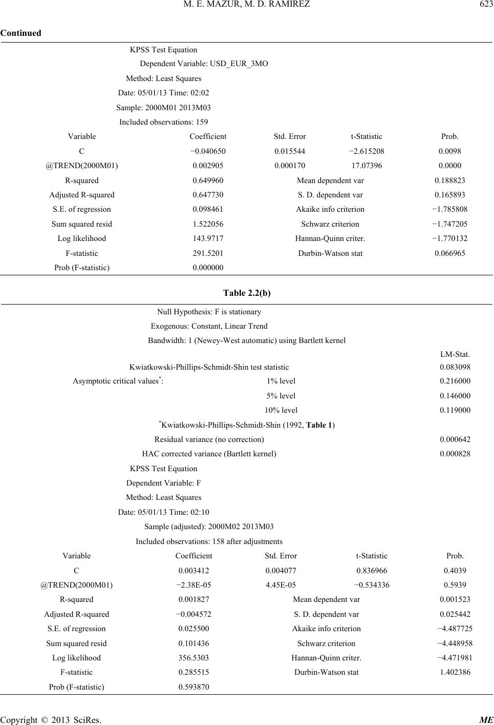

M. E. MAZUR, M. D. RAMIREZ 623

Continued

KPSS Test Equation

Dependent Variable: USD_EUR_3MO

Method: Least Squares

Date: 05/01/13 Time: 02:02

Sample: 2000M01 2013M03

Included observations: 159

Variable Coefficient Std. Error t-Statistic Prob.

C −0.040650 0.015544 −2.615208 0.0098

@TREND(2000M01) 0.002905 0.000170 17.07396 0.0000

R-squared 0.649960 Mean dependent var 0.188823

Adjusted R-squared 0.647730 S. D. dependent var 0.165893

S.E. of regression 0.098461 Akaike info criterion −1.785808

Sum squared resid 1.522056 Schwarz criterion −1.747205

Log likelihood 143.9717 Hannan-Quinn criter. −1.770132

F-statistic 291.5201 Durbin-Watson stat 0.066965

Prob (F-statistic) 0.000000

Table 2.2(b)

Null Hypothesis: F is stationary

Exogenous: Constant, Linear Trend

Bandwidth: 1 (Newey-West automatic) using Bartlett kernel

LM-Stat.

Kwiatkowski-Phillips-Schmidt-Shin test statistic 0.083098

Asymptotic critical values*: 1% level 0.216000

5% level 0.146000

10% level 0.119000

*Kwiatkowski-Phillips-Schmidt-Shin (1992, Table 1)

Residual variance (no correction) 0.000642

HAC corrected variance (Bartlett kernel) 0.000828

KPSS Test Equation

Dependent Variable: F

Method: Least Squares

Date: 05/01/13 Time: 02:10

Sample (adjusted): 2000M02 2013M03

Included observations: 158 after adjustments

Variable Coefficient Std. Error t-Statistic Prob.

C 0.003412 0.004077 0.836966 0.4039

@TREND(2000M01) −2.38E-05 4.45E-05 −0.534336 0.5939

R-squared 0.001827 Mean dependent var 0.001523

Adjusted R-squared −0.004572 S. D. dependent var 0.025442

S.E. of regression 0.025500 Akaike info criterion −4.487725

Sum squared resid 0.101436 Schwarz criterion −4.448958

Log likelihood 356.5303 Hannan-Quinn criter. −4.471981

F-statistic 0.285515 Durbin-Watson stat 1.402386

Prob (F-statistic) 0.593870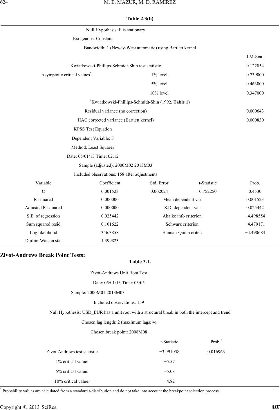

M. E. MAZUR, M. D. RAMIREZ

624

Table 2.3(b)

Null Hypothesis: F is stationary

Exogenous: Constant

Bandwidth: 1 (Newey-West automatic) using Bartlett kernel

LM-Stat.

Kwiatkowski-Phillips-Schmidt-Shin test statistic 0.122854

Asymptotic critical values*: 1% level 0.739000

5% level 0.463000

10% level 0.347000

*Kwiatkowski-Phillips-Schmidt-Shin (1992, Table 1)

Residual variance (no correction) 0.000643

HAC corrected variance (Bartlett kernel) 0.000830

KPSS Test Equation

Dependent Variable: F

Method: Least Squares

Date: 05/01/13 Time: 02:12

Sample (adjusted): 2000M02 2013M03

Included observations: 158 after adjustments

Variable Coefficient Std. Error t-Statistic Prob.

C 0.001523 0.002024 0.752250 0.4530

R-squared 0.000000 Mean dependent var 0.001523

Adjusted R-squared 0.000000 S.D. dependent var 0.025442

S.E. of regression 0.025442 Akaike info criterion −4.498554

Sum squared resid 0.101622 Schwarz criterion −4.479171

Log likelihood 356.3858 Hannan-Quinn criter. −4.490683

Durbin-Watson stat 1.399823

Zivot-Andrews Break Point Tests: Table 3.1.

Zivot-Andrews Unit Root Test

Date: 05/01/13 Time: 03:05

Sample: 2000M01 2013M03

Included observations: 159

Null Hypothesis: USD_EUR has a unit root with a structural break in both the intercept and trend

Chosen lag length: 2 (maximum lags: 4)

Chosen break point: 2008M08

t-Statistic Prob.*

Zivot-Andrews test statistic −3.991058 0.016963

1% critical value: −5.57

5% critical value: −5.08

10% critical value: −4.82

* Probability values are calculated from a standard t-distribution and do not take into account the breakpoint selection process.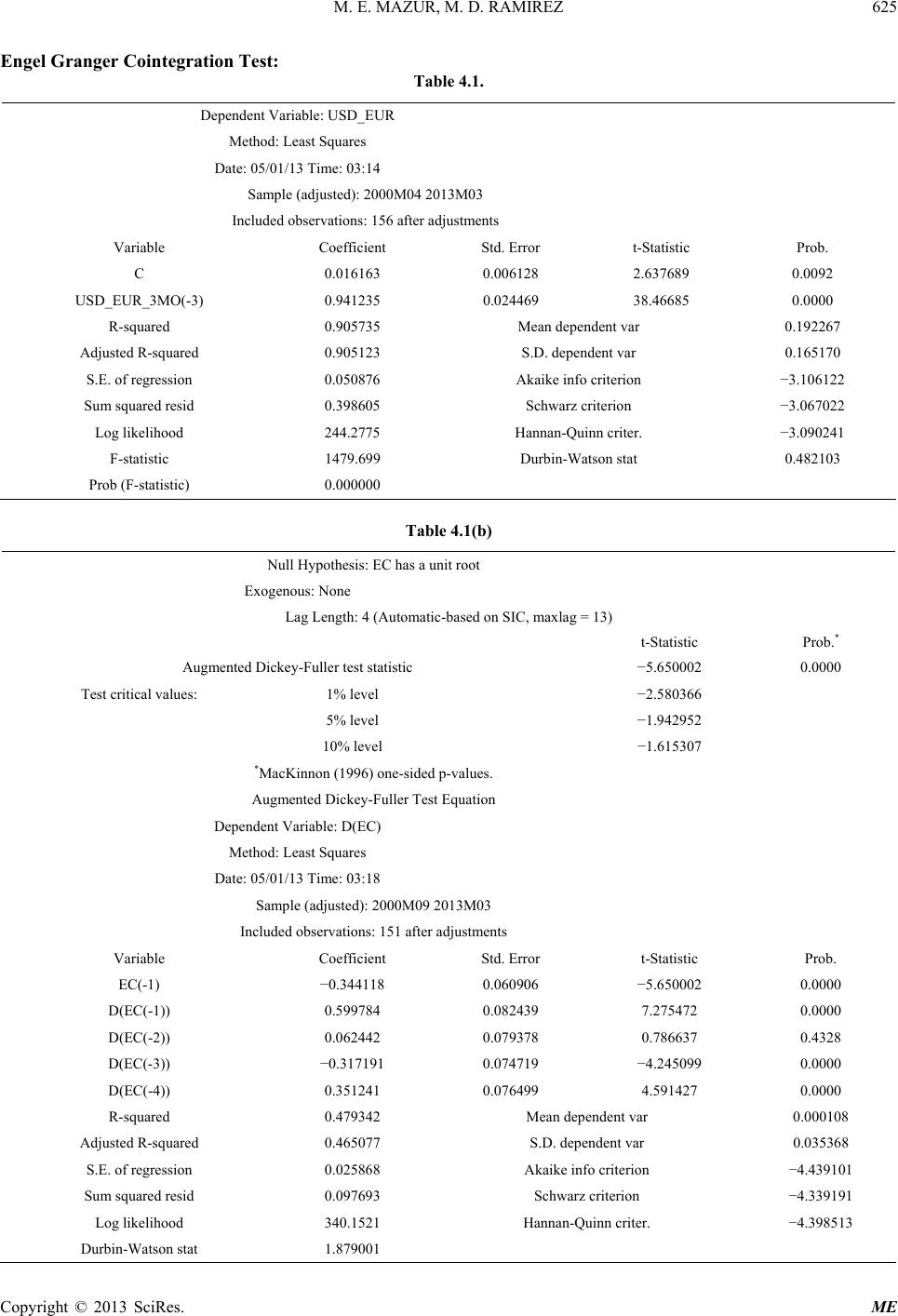

M. E. MAZUR, M. D. RAMIREZ 625

Engel Granger Cointegration Test: Table 4.1.

Dependent Variable: USD_EUR

Method: Least Squares

Date: 05/01/13 Time: 03:14

Sample (adjusted): 2000M04 2013M03

Included observations: 156 after adjustments

Variable Coefficient Std. Error t-Statistic Prob.

C 0.016163 0.006128 2.637689 0.0092

USD_EUR_3MO(-3) 0.941235 0.024469 38.46685 0.0000

R-squared 0.905735 Mean dependent var 0.192267

Adjusted R-squared 0.905123 S.D. dependent var 0.165170

S.E. of regression 0.050876 Akaike info criterion −3.106122

Sum squared resid 0.398605 Schwarz criterion −3.067022

Log likelihood 244.2775 Hannan-Quinn criter. −3.090241

F-statistic 1479.699 Durbin-Watson stat 0.482103

Prob (F-statistic) 0.000000

Table 4.1(b)

Null Hypothesis: EC has a unit root

Exogenous: None

Lag Length: 4 (Automatic-based on SIC, maxlag = 13)

t-Statistic Prob.*

Augmented Dickey-Fuller test statistic −5.650002 0.0000

Test critical values: 1% level −2.580366

5% level −1.942952

10% level −1.615307

*MacKinnon (1996) one-sided p-values.

Augmented Dickey-Fuller Test Equation

Dependent Variable: D(EC)

Method: Least Squares

Date: 05/01/13 Time: 03:18

Sample (adjusted): 2000M09 2013M03

Included observations: 151 after adjustments

Variable Coefficient Std. Error t-Statistic Prob.

EC(-1) −0.344118 0.060906 −5.650002 0.0000

D(EC(-1)) 0.599784 0.082439 7.275472 0.0000

D(EC(-2)) 0.062442 0.079378 0.786637 0.4328

D(EC(-3)) −0.317191 0.074719 −4.245099 0.0000

D(EC(-4)) 0.351241 0.076499 4.591427 0.0000

R-squared 0.479342 Mean dependent var 0.000108

Adjusted R-squared 0.465077 S.D. dependent var 0.035368

S.E. of regression 0.025868 Akaike info criterion −4.439101

Sum squared resid 0.097693 Schwarz criterion −4.339191

Log likelihood 340.1521 Hannan-Quinn criter. −4.398513

Durbin-Watson stat 1.879001

M. E. MAZUR, M. D. RAMIREZ

626

Table 4.2.

Dependent Variable: USD_EUR

Method: Least Squares

Date: 05/01/13 Time: 03:12

Sample (adjusted): 2000M04 2013M03

Included observations: 159

Variable Coefficient Std. Error t-Statistic Prob.

C 0.000525 0.000377 −1.391272 0.1661

USD_EUR_3MO 1.000492 0.001502 666.1035 0.0000

R-squared 0.999646 Mean dependent var 0.188391

Adjusted R-squared 0.999644 S.D. dependent var 0.166004

S.E. of regression 0.003132 Akaike info criterion −8.681760

Sum squared resid 0.001540 Schwarz criterion −8.643158

Log likelihood 692.1999 Hannan-Quinn criter. −8.666084

F-statistic 443693.9 Durbin-Watson stat 0.157920

Prob (F-statistic) 0.000000

Table 4.2(b)

Null Hypothesis: EC2 has a unit root

Exogenous: None

Lag Length: 1 (Automatic-based on SIC, maxlag = 13)

t-Statistic Prob.*

Augmented Dickey-Fuller test statistic −2.402287 0.0162

Test critical values: 1% level −2.579774

5% level −1.942869

10% level −1.615359

*MacKinnon (1996) one-sided p-values.

Augmented Dickey-Fuller Test Equation

Dependent Variable: D(EC2)

Method: Least Squares

Date: 05/01/13 Time: 03:21

Sample (adjusted): 2000M03 2013M03

Included observations: 157 after adjustments

Variable Coefficient Std. Error t-Statistic Prob.

EC2(−1) −0.073882 0.030755 −2.402287 0.0175

D(EC2(−1)) −0.254660 0.076717 −3.319472 0.0011

R-squared 0.114773 Mean dependent var 3.80E − 05

Adjusted R-squared 0.109062 S.D. dependent var 0.001247

S.E. of regression 0.001177 Akaike info criterion −10.63914

Sum squared resid 0.000215 Schwarz criterion −10.60020

Log likelihood 837.1723 Hannan-Quinn criter. −10.62332

Durbin-Watson stat 2.064020