Estimation of Location Parameter from Two Biased Samples

doi:10.4236/am.2013.49171

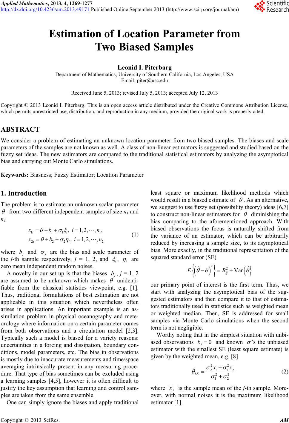Applied Mathematics, 2013, 4, 1269-1277

http://dx.doi.org/10.4236/am.2013.49171 Published Online September 2013 (http://www.scirp.org/journal/am)

Estimation of Location Parameter from

Two Biased Samples

Leonid I. Piterbarg

Department of Mathematics, University of Southern California, Los Angeles, USA

Email: [email protected]

Received June 5, 2013; revised July 5, 2013; accepted July 12, 2013

which permits unrestricted use, distribution, and reproduction in any medium, provided the original work is properly cited.

ABSTRACT

We consider a problem of estimating an unknown location parameter from two biased samples. The biases and scale

parameters of the samples are not known as well. A class of non-linear estimators is suggested and studied based on the

fuzzy set ideas. The new estimators are compared to the traditional statistical estimators by analyzing the asymptotical

bias and carrying out Monte Carlo simulations.

Keywords: Biasness; Fuzzy Estimator; Location Parameter

1. Introduction

The problem is to estimate an unknown scalar parameter



from two different independent samples of size n1 and

n2

111

222

, 1,2,,,

, 1,2,,

ii

1

2

x

bi n

x

bi





 

 



n

(1)

where

j

b and

j



are the bias and scale parameter of

the j-th sample respectively, j = 1, 2, and i



, i



are

zero mean independent random noises.

A novelty in our set up is that the biases

j

b, j = 1, 2

are assumed to be unknown which makes



unidenti-

fiable from the classical statistics viewpoint, e.g. [1].

Thus, traditional formulations of best estimation are not

applicable in this situation which nevertheless often

arises in applications. An important example is an as-

similation problem in physical oceanography and mete-

orology where information on a certain parameter comes

from both observations and a circulation model [2,3].

Typically such a model is biased for a variety reasons:

uncertainties in a forcing and dissipation, boundary con-

ditions, model parameters, etc. The bias in observations

is mostly due to inaccurate measurements and time/space

averaging intrinsically present in any measuring proce-

dure. That type of bias sometimes can be excluded using

a learning samples [4,5], however it is often difficult to

justify the key assumption that learning and control sam-

ples are taken from the same ensemble.

One can simply ignore the biases and apply traditional

least square or maximum likelihood methods which

would result in a biased estimate of



. As an alternative,

we suggest to use fuzzy set (possibility theory) ideas [6,7]

to construct non-linear estimators for



diminishing the

bias comparing to the aforementioned approach. With

biased observations the focus is naturally shifted from

the variance of an estimator, which can be arbitrarily

reduced by increasing a sample size, to its asymptotical

bias. More exactly, in the traditional representation of the

squared standard error (SE)











22

ˆ

ˆˆ

VarEB







our primary point of interest is the first term. Thus, we

start with analyzing the asymptotical bias of the sug-

gested estimators and then compare it to that of estima-

tors traditionally used in statistics such as weighted mean

or weighted median. Then, SE is addressed for small

samples via Monte Carlo simulations when the second

term is not negligible.

Worthy noting that in the simplest situation with unbi-

ased observations 0

j

b



and known



’s the unbiased

estimator with the smallest SE (least square estimate) is

given by the weighted mean, e.g. [8]

22

211 2

22

12

ˆLS

x







 (2)

where

j

x

is the sample mean of the j-th sample. More-

over, with normal noises it is the maximum likelihood

estimator [1].

C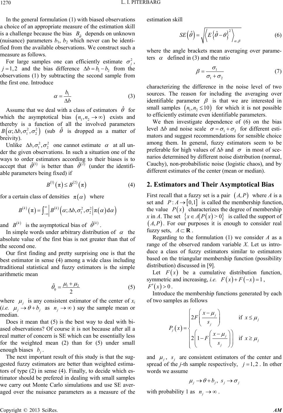

L. I. PITERBARG

1270

In the general formulation (1) with biased observations

a choice of an appropriate measure of the estimation skill

is a challenge because the bias ˆ

B



depends on unknown

(nuisance) parameters b1, b2 which never can be identi-

fied from the available observations. We construct such a

measure as follows.

For large samples one can efficiently estimate 2

j



,

and the bias difference 12

from the

observations (1) by subtracting the second sample from

the first one. Introduce

1, 2jbbb 

1

b



 (3)

Assume that we deal with a class of estimators ˆ



for

which the asymptotical bias exists and

thereby is a function of all the involved parameters



12

,nn





22

12

;,,Bb





 (sub ˆ



is dropped as a matter of

breivity).

Unlike 22

12

,,b



 one cannot estimate



all un-

der the given observations. In such a situation one of the

ways to order estimators according to their biases is to

accept that



1

ˆ

at



is better than



ˆ2



(under the identifi-

able parameters being fixed) if



12

πBBπ (4)

for a certain class of densities



π



where







22

12

π;,, πd

kk

BBb



 









and is the asymptotical bias of



k

B



ˆk



.

In simple words under arbitrary distribution of



the

absolute value of the first bias is not greater than that of

the second one.

Our first finding and pretty surprising one is that the

best estimator in sense (4) among a wide class including

traditional statistical and fuzzy estimators is the simple

arithmetic mean

12

0

ˆ

2







 (5)

where

j



is any consistent estimator of the center of xi

(i.e.

j

b





 as ) say the sample mean or

median.

j

n

Does it mean that (5) is the best way to deal with bi-

ased observations? Of course it is not because after all a

real matter of concern is SE which can be essentially less

for the weighted mean (2) than for (5) under small

enough biases

j

b.

The next important result of this study is that the sug-

gested fuzzy estimators are better than weighted estima-

tors of type (2) in sense (4). Finally, to decide which es-

timator should be prefered in dealing with small samples

we carry out Monte Carlo simulations and use SE aver-

aged over the nuisance parameters as a measure of the

estimation skill

 

2

,

ˆˆ

SE E







 (6)

where the angle brackets mean averaging over parame-

ters



defined in (3) and the ratio

1

12







 (7)

characterizing the difference in the noise level of two

sources. The reason for including the averaging over

identifiable parameter



is that we are interested in

small samples





1

12 for which it is not possible

to efficiently estimate even identifiable parameters.

, 0nn

We then investigate dependence of (6) on the bias

level ∆b and noise scale 12





 for different esti-

mators and suggest recommendations for sensible choice

among them. In general, fuzzy estimators seem to be

preferable for high values of ∆b and



in most of sce-

narios determined by different noise distribution (normal,

Cauchy), non-probabilistic noise (logistic chaos), and by

different estimates of the center (mean or median).

2. Estimators and Their Asymptotical Bias

First recall that a fuzzy set is a pair



,



A

P where A is a

set and





:0,PA1 is called the membership function,

the value





Px characterizes the degree of membership

x in A. The set









>0PxxA is called the support of





,

A

P. For our purposes it is enough to consider real

fuzzy sets,

A

R.

Regarding to the formulation (1) we consider A as a

range of the observed random variable X. Let us intro-

duce a class of fuzzy estimators similar to estimators

based on the triangular membership function (possibility

distribution) discussed in [9].

Let





F

x be a cumulative distribution function,

symmetric and increasing, i.e. ,

 

1FxF x





Fx

0.

Introduce the membership functions generated by each

of two samples as follows



2i

21if

jf

j

x

Fx

s

Px

x

Fx

s







































and

j



,

j

s

are consistent estimators of the center and

spread of the j-th sample respectively, . In other

words we assume

1, 2j

,

j

jj

bs j







with probability 1 as .

j

n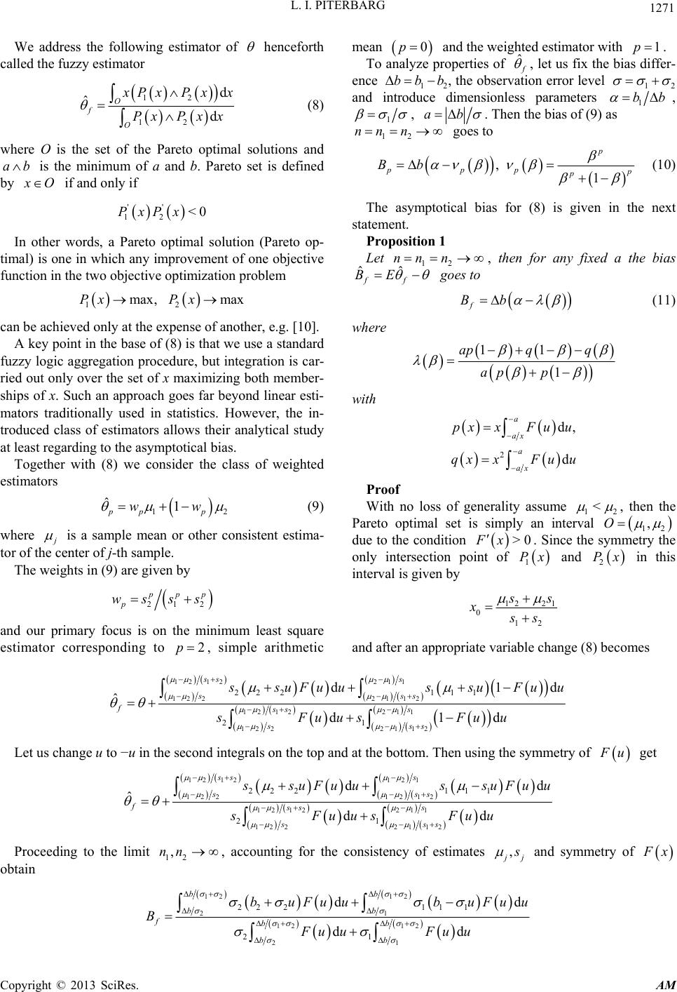

L. I. PITERBARG

1271

mean





0p



and the weighted estimator with 1p



. We address the following estimator of



henceforth

called the fuzzy estimator To analyze properties of ˆ

f



, let us fix the bias differ-

ence 12

bb b



, the observation error level 12









and introduce dimensionless parameters 1

bb





,

1







, ab



 . Then the bias of (9) as

12

nn n



 goes to

 



 

12

d

ˆ

d

O

f

O

x

Px Px x

PxP xx









 (8)

where O is the set of the Pareto optimal solutions and

is the minimum of a and b. Pareto set is defined

by

ab

x

O if and only if



 

,

1

p

ppp

p

Bb



  



  (10)

The asymptotical bias for (8) is given in the next

statement.









''

12

<0PxPx

Proposition 1

In other words, a Pareto optimal solution (Pareto op-

timal) is one in which any improvement of one objective

function in the two objective optimization problem

Let 12

nn n





ˆf

, then for any fixed a the bias

ˆf

BE





 goes to







f

Bb







  (11)

 

12

max, maxPx Px

can be achieved only at the expense of another, e.g. [10]. where

A key point in the base of (8) is that we use a standard

fuzzy logic aggregation procedure, but integration is car-

ried out only over the set of x maximizing both member-

ships of x. Such an approach goes far beyond linear esti-

mators traditionally used in statistics. However, the in-

troduced class of estimators allows their analytical study

at least regarding to the asymptotical bias.





 

 





11

1

ap q q

ap p





 

 



with

 

2

d,

d

a

ax

a

ax

pxxFu u

qxxFu u







Together with (8) we consider the class of weighted

estimators Proof





1

ˆ1

pp p

ww With no loss of generality assume 12

<



, then the

Pareto optimal set is simply an interval





12

,O





due to the condition





>0Fx



1

Px

. Since the symmetry the

only intersection point of and in this

interval is given by





2

Px



2

 

 (9)

where

j



is a sample mean or other consistent estima-

tor of the center of j-th sample.

The weights in (9) are given by



21 2

p

pp

p

wsss 12 21

0

12

s

xss







and our primary focus is on the minimum least square

estimator corresponding to , simple arithmetic

2pand after an appropriate variable change (8) becomes

























12 12211

12221 12

12 12211

12221 12

22 2111

21

d1

ˆ

d1d

ss s

sss

fss s

sss

d

s

suFu ussuFuu

sFuus Fuu

 





 



 



 

 



Let us change u to −u in the second integrals on the top and at the bottom. Then using the symmetry of





F

u get





















12 12121

12212 12

12 12211

1222112

22 2111

21

dd

ˆ

dd

ss s

sss

fss s

sss

s

suFu ussuFuu

sFuusFuu

 

 





 



 



 

 



Proceeding to the limit , accounting for the consistency of estimates

12

,nn ,

j

s



and symmetry of





F

x

obtain











12 12

21

12 12

21

22211 1

21

dd

bb

fbb

bb

buFuu buFu

B

Fu uFu u

 



 



 



 



 



 





u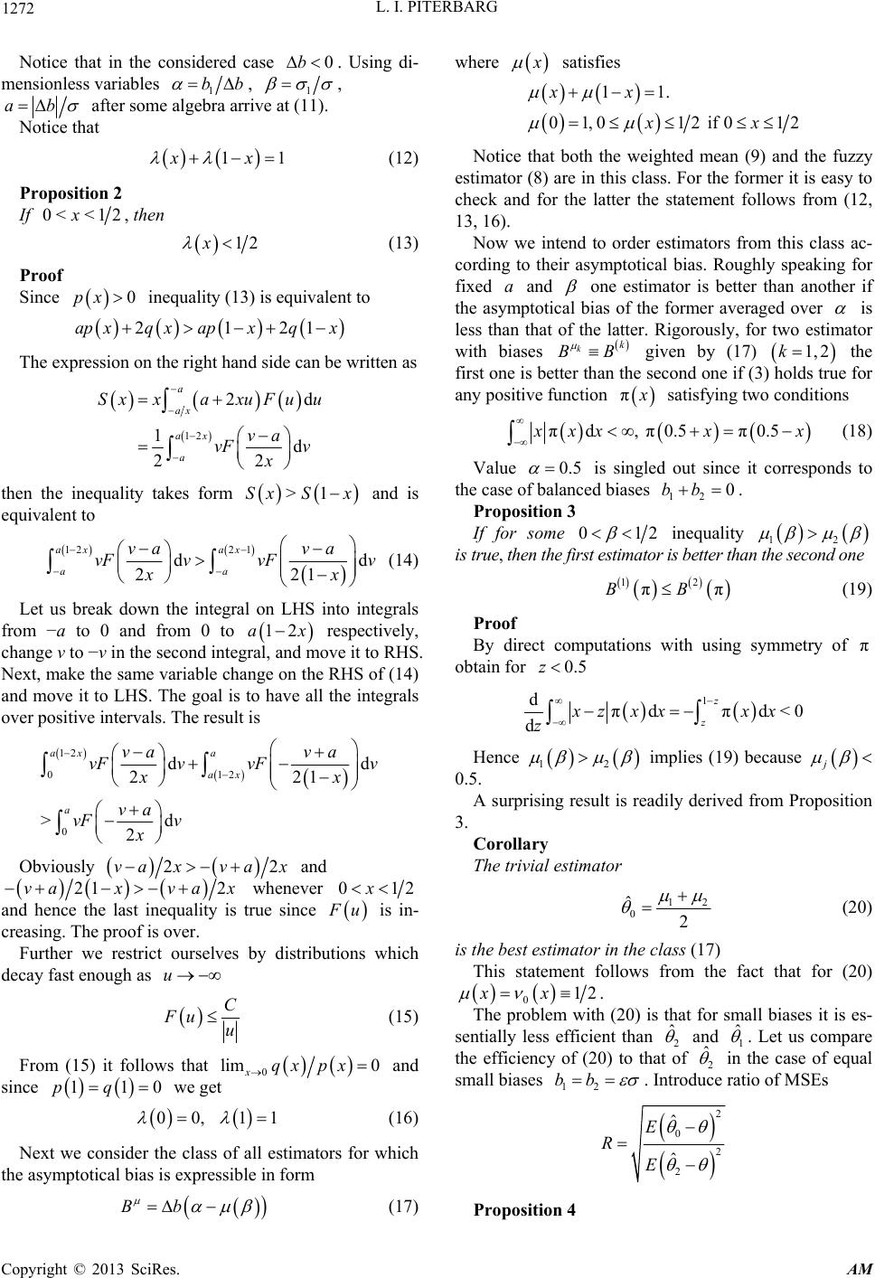

L. I. PITERBARG

1272

Notice that in the considered case . Using di-

mensionless variables

0b

1

bb



, 1





,

ab



 after some algebra arrive at (11).

Notice that







1xx



1 (12)

Proposition 2

If 0< <12x, then



12x



 (13)

Proof

Since inequality (13) is equivalent to



0px

 





2121apx qxapx qx



The expression on the right hand side can be written as

 



12

2d

1d

22

a

ax

a

SxxaxuFu u

va

vF v

x















then the inequality takes form and is

equivalent to

 

>1Sx Sx

 



122 1

d

221

ax ax

aa

va va

vFv vFv

x











 



 



d

x





x

(14)

Let us break down the integral on LHS into integrals

from −a to 0 and from 0 to respectively,

change v to −v in the second integral, and move it to RHS.

Next, make the same variable change on the RHS of (14)

and move it to LHS. The goal is to have all the integrals

over positive intervals. The result is



12a



12

012

0

dd

22

>d

2

ax a

ax

a

va va

vFv vFv

xx

va

vF v

x













 



 















1

Obviously

 

22va xva x and



21 2vaxva x  whenever 01x2



and hence the last inequality is true since





F

u is in-

creasing. The proof is over.

Further we restrict ourselves by distributions which

decay fast enough as

u



C

Fu u

 (15)

From (15) it follows that

 

0

lim 0

xqx px





and

since we get

 

11pq0









00,1



1 (16)

Next we consider the class of all estimators for which

the asymptotical bias is expressible in form



Bb





 





x



satisfies

(17)

where









 

11.

01,0 12 if 012

xx





 

Notice that both the weighted mean (9) and e fuzzy

estimator (8) are in this class. For the former it is easy to

ch

th

eck and for the latter the statement follows from (12,

13, 16).

Now we intend to order estimators from this class ac-

cording to their asymptotical bias. Roughly speaking for

fixed a and



one estimator is better than another if

the asymptotical bias of the former averaged over



is

less than that of the latter. Rigorously, for two estimator

with biases



kk

BB





given by (17)



1, 2kthe

first one is better than the second one if (3) holds true for

any positive fu

nction





π

x

satisfying two conditions

 

πd, π0.5 π0.5

x

xxx x









 (18)

Value 0.5





of bala

ition 3

is singled out since it corresp

the case nced biases

onds to

12

0bb.

Propos

If for some 012







inequality





12







he second one is estimato true, then the first r is better than t



12

ππB



Proof

By direct computations with usin

ob

B (19)

g symmetry of π

tain for 0.5z



 

1

dπdπd<0

d

z

xxxx





z

xz

z 



Hence









12

 

 implies (19) because





j





0.5.

ising result is rA surpreadily derived from Proposition

3.

Corolla ry

The trivial estimator

12

0

ˆ

2







 (20)

is the best estimator in the class (17

This statement follows from the fact that for

)

(20)









012xx



.

The problem with (20) is that for small biases it is es-

han ˆ

sentially less efficient t2



and ˆ

1



. Let us compare

the efficiency of (20) to that of 2

ˆ



in the case of equal

small biases 12

bb







. Introduce ratio of MSEs



2

0

ˆ

E

2

ˆ

R

E







Proposition 4



L. I. PITERBARG 1273

For any large

(21)

whenever

>0C

RC

11



 111 1

or

2 122 1

CC





 

(22)

and

2



2

22

222

2

22

141

41 1

C









 







(23)

oof

Let

Pr



2

214s



 and



 



2

22

11t





2

then (21) becomes

2

C

2

s

t





or

2

21

s

tC

C









(24)

Inequality is equivalent to (23) and then

turns in

xample assume C = 2, then (20) holds true if β >

0.7887 or β < 0.2113. Then for β =

< 0.2594.

orth to co

20stC

(22). (24)

For e

0.1 we have R > 2 if ε

Thus it is wmpare the suggested fuzzy esti-

mators with 2

ˆ



and 1

ˆ



. For that purpose we need an-

other representation for



appearing in (11)

 

 



1TxTx

xx





 (25)

1

apxpx

where

 

2dTxxauFuu



a

ax



Since the denominator in (25) is positiv

following statement gives conditions for for the fuzzy

r to dominate

e for all x the

estimato 1

ˆ



.

Proposition 5

 

>, 0,12xxx



 (26)

if and only if

 

1Txx > 0, 0,12T x (27)

e possibility distribuFor example if thtion is given by



1

Pu u





(28)

which corresponds to









0.51, <0u, then













 

Fu u

(27) is fulfilled. Indeed, for (28)

2

1l

n1

1

bx

xx



 







Then for any fixed

21

ln1 ,

bx





,1txbTx Tx

1

a

ba



one gets





,0 0tx







0,1 2x

and









12 0

21 1

bx

t

bxbxxbx











which implies (27).

t always fue triangle

bership function defined by the cumulative prob-

ability distribution function

Condition (27) is nolfilled for th

mem



1if

0.5

0if

uqu

q

Fu

uq

0













where q is a fixed quantile. Indeed, direct computations

yield [11].

Proposition 6









 





 



 

32

2

32

2

1231 12

1211

312

11

1ifmin 1,11

3

132

1

ifmax 1,11

12 1

if 111

xxx

xx

x

xx x

xx

x









if 11 1x























 





















where







qa





.

be deriIt canved from that statement that (26) holds

true if and only if 12



 while for 173



 the

opposite relation holds true:



x



 for all 01x2



.

In the intermediate case 73 1



2 the difference





x





changes the sign once in



0,1 2. If 1





then two samples are incompatible.

These conclusions are illustrated in Figure 1 by plot-

ting the difference





d

x

xx





 for the triangular

membership function (left and middle panel) anr

membership (28) (right panel2

d fo

). If 1



 then for sure

73





and hence





d0x



for 1xt panel). If

23

2 (lef

er







 then two options are possible eith



dx

or

0





d

x

changes the sign once (cen

tral pane l). Finally

L. I. PITERBARG

1274

Figure 1. The difference λ(x) − x vs x. 1) Triangle membership, 1 < γ < 2; 2) Triangle membership, 2 < γ < 3; 3) Membership

given by (28), 0.5 ≤ a ≤ 5.

for membership (2) for all

a.

However, it can be s[9], that



d0x

hown





p



x



 (29)



2

x



 when for all



0,1 2x thereby the fuzzy triangle estimator is better

than 2

ˆ



in sense (19).

012x



. Then







1

12

1,12

p

Gxa



 

 dx

(29) the region always occupies more

than a half

Nex efine another quantitative for

asy to evaluate,

un he parame

interest

t, dcharacteristic

comparing asymptotical biases which is eThus under G



like



πB. First define the space of tters of . In particular, for



1

x





.125 and fo



,1232, 01

 

 

The range for



is founded in [9]. Then introduce

the diffe of biases for the mentioned estimators de-

fined by

thetegral

on the right side is equalr

in

hand to 0



erenc

functions 1



x



and



2

x



respectively



12

,BBB







and define

 



12 , 0GB

 

  ,



Obviously the area of equals 2 a hence the first

estimator can be viewebetter than the second one

he area of exceeds 1. This excess is

quantified in the nextnt.

Proposition 7



d as

12

G

stateme

nd

whenever t

If

 

12

x



, 012 then x

 



12

1212

0

11 d1Gxxx



 



Indeed, the solution of







12

<

x





 



is

equivalent to

 



12

>2xx

 

 from which the

stent readily follows.

The following proposition gives a rough estimate of

improving a fuzzy estimator comparing to any weighted

m

atem

ean (9). Set

 



, ,GB,

fp

B











 

Corolla ry

Let for some fixed a

 



2

1

x

xxx



 it is ln240.1733. The

latter follows from

 

12

2

0d1lxx







rticular, the area of a region in where the

bias of the fuzzy estimator (28) is less thaat of

n24

In pa

n 1

ˆ



th is

greater than 1.125. While the area of a on in regi



wathere the fuzzy triangle estimor is better than 2

ˆ



is

greater than 1733. 1.

3. Simulations

The goal of the performed simulations is to compare the

efficiency of different estimators underfferent noise

distributions.

di

Now the asymptotical bias is not of primary

concern, but rather the relative standard error

 

2

1.5 1

20.5 0

1

ˆˆdd

2

SE E



 











is addressed under small samples.

o fuzzy estimators (8), first, deter-

1) and, second, determined by

We examine tw

mined by (28) (Fuzzy



0.5eu

Pu



 (Fuzzy 2) and three weighted estimators

0

ˆ



, 1

ˆ



and 2

ˆ



given by (9).

Sample sizes 12

10nn



 and number of Monte

Carlo trials M = 100 for each mesh



,





are kept the

same for all ex

First, normal noise is tested with

periments.

j

x



, i.e. the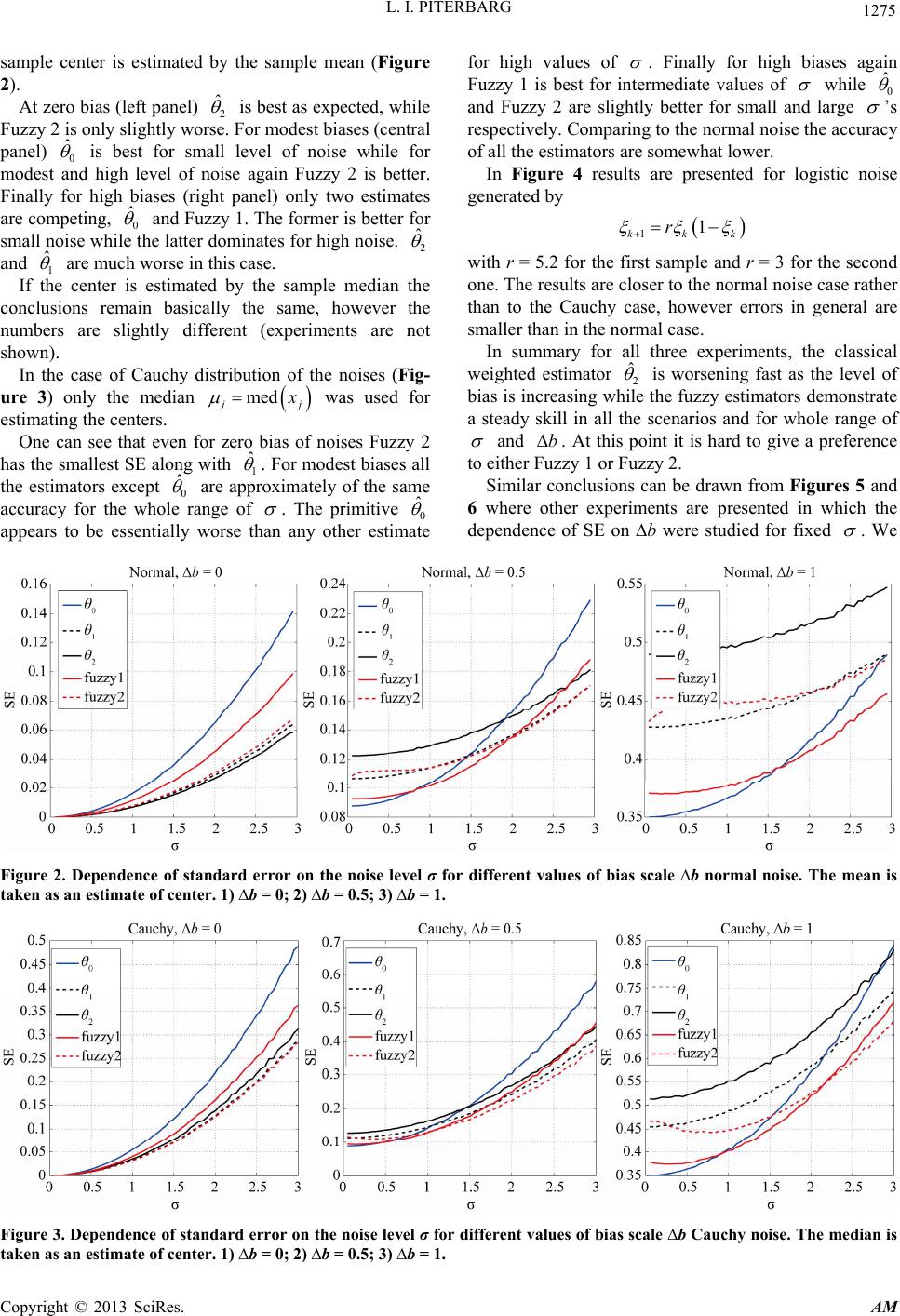

L. I. PITERBARG 1275

sample center is estimated by the sample mean (Figure

2).

At zero bias (left panel) 2

ˆ



is best as expected, while

modest biases (central

pa

Fuzzy 2 is only slightly worse. For

nel) 0

ˆ



is best for small level of noise while for

modest and high level of noise again Fuzzy 2 is better.

h biases (right panel) only two estimates

peting ˆ

Finally hig

are co,

for

m0



and Fuzzy 1. The former is better for

small noise while the latter dominates for high noise. 2

ˆ



and 1

ˆ



are much worse in this case.

If the center is estimated by

the sample median the

coe, how

n).

stri

nclusions remain basically the samever the

numbers are slightly different (experiments are not

show

In the case of Cauchy dibution of the noises (Fig-

ure 3) only the median



med

j

x



 was used for

estimati the centers.

One can see that even for zero bias of noises Fuzzy 2

has the smallest SE along with 1

ˆ

ng



. For modest biases all

the estimators except 0

ˆ



are approximately of the same

accuracy for the whole range of



. The primitive 0

ˆ



appe to be essentially worse than aarsny other estim ate

for high values of



. Finally for high biases again

Fuzzy 1 is best for intermediate values of



while 0

ˆ



and Fuzzy 2 are slightly better for small and large



’s

respectively. Comparing to the normal noise the accuracy

of all the estimators are somewhat lower.

In Figure 4 results are presented for logistic noise

generated by



11

kk

rk







with r = 5.2 for the first sample and r = 3 for the second

one. The results are closer to the normal noise case rather

than to the Cauchy case, however errors in general are

smaller than in the normal case.

In summary for all three experiments, the classical

weighted estimator 2

ˆ



is worsening fast as the level of

bias is increasing while the fuzzy estimators demonstrate

a steady skill in all the scenarios and for whole range of



and b



. At this point it is hard to give a preference

to either Fuzzy 1 or Fuzzy 2.

Similar conclusions can be drawn from Figures 5 and

6 where other experiments are presented in which the

dependence of SE on ∆b were studied for fixed



. We

Figure 2. Dependence of standard error on the noise level σ for different values of bias scale ∆b normal noise. The mean is

taken as an estimate of center. 1) ∆b = 0; 2) ∆b = 0.5; 3) ∆b = 1.

Figure 3. Dependence of standard error on the noise level σ for different values of bias scale ∆b Cauchy noise. The median is

taken as an estimate of center. 1) ∆b = 0; 2) ∆b = 0.5; 3) ∆b = 1.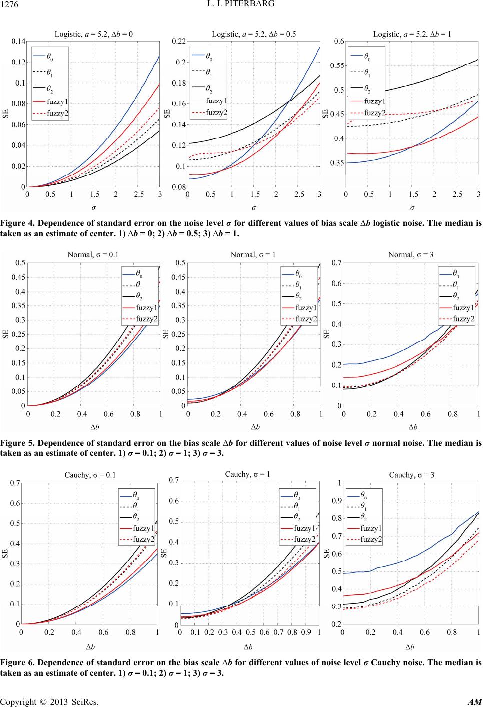

L. I. PITERBARG

1276

Figure 4. Dependence of standard error on the noise level σ for different values of bias scale ∆b logistic noise. The median is

taken as an estimate of center. 1) ∆b = 0; 2) ∆b = 0.5; 3) ∆b = 1.

Figure 5. Dependence of standard error on the bias scale ∆b for different values of noise level σ normal noise. The median is

taken as an estimate of center. 1) σ = 0.1; 2) σ = 1; 3) σ = 3.

Figure 6. Dependence of standard error on the bias scale ∆b for different values of noise level σ Cauchy noise. The median is

taken as an estimate of center. 1) σ = 0.1; 2) σ = 1; 3) σ = 3.

L. I. PITERBARG

1277

want to stress two of them, first, for high



e and, second,

Fuzzy 2 is

uniformly better than any other estimat0

ˆ



is not appropriate for such values of



regardless

noise distribution.

4. Conclusions and Discussion

A majority of studies in estimating a location parameter

address, first, linear functionals of either the original

sample or its ranking, e.g. [11], and, second, unbiased

observations. Here a class of essentially nonlinear esti-

mators is suggested based on the fuzzy set theory ideas to

handle biased observations coming from two different

sources. Because any analytical investigation of the

standard error for highly non-linear functions of sample

an the classical least square estimator.

r

are estimator and

N00014-11-1-0369 and NSF under grant CMG-1025453

is greatly appreciated.

REFERENCES

[1] G. Casella and R. Berger, “Statistical Inference,” 2nd

Edition, Brooks/Cole, Pacific Grove, 1990.

[2] M. Ghil, “Meteorological Data Assimilation for Ocean-

ographers. Part 1; Description and Theoretical Frame-

work,” Dynamics of Atmospheres and Oceans, Vol. 13,

No. 2, 1989, pp. 171-218.

doi:10.1016/0377-0265(89)90040-7

the

[3] P. Malanotte-Rizzoli, “Modern Approaches to Data As-

similation in Ocean Modeling,” Elsevier, Amsterdam,

1996.

[4] T. Krishnamurti, C. Kishtawal, Z. Zhang, T. Larow, D.

casts for Weather and Seasonal Climate,” Journal of Cli-

is hard, we concentrated on, first, analytical studying the

asymptotical bias of the suggested estimators and, second,

onte Carlo simulations for small samples with the tra

Bachiochi and E. Williford, “Multimodel Ensemble Fore-

M-

ditional standard error as an efficiency measure.

Conclusions from both studies are similar. Regarding

the symptotical bias, the considered fuzzy estimators are

uniformly better th

mate, Vol. 13, No. 8, 2000, pp. 4196-4216.

doi:10.1175/1520-0442(2000)013<4196:MEFFWA>2.0.

CO;2

[5] F. J. Lenartz, M. Beckers, J. Chiggiato, B. Mourre, C.

and M. Rixen, “Super Ensem-

Wave Forecast: Performance

Troupin, L. Vandenbulcke

ble Techniques Applied to

As for small samples, the new estimators are of highe

accuracy than the traditional least squand Limitations,” Ocean Science, Vol. 6, No. 3, 2010, pp.

595-604. doi:10.5194/os-6-595-2010

[6] D. Dubois and H. Prade, “Possibilty Theory,” Plenum

Press, New York, L

its modifications for essential bias and high level of noise.

Moreover, even for small bias, the fuzzy estimators are

only slightly worse than the optimal one.

Unexpectedly, the primitive arithmetic mean succes-

fully competes with fuzzy estimators for essential biases

and modest noise level, but it is of little help for high

level of noise or negligable biases.

Notice that the developed fuzzy estimators are highly

non-linear functionals of observations and apparently are

more appropriate for estimating parameters in non-linear

complex systems.

We tested only two estimators from a wide class in-

tro

ondon, 1988.

doi:10.1007/978-1-4684-5287-7

[7] G. Shafer, “A Evidence,” Prince-

Independent

Mathematical Theory of

ton University Press, Hoboken, 1976.

[8] T. P. Hill and J. Miller, “How to Combine

Data Sets for the Same Quantity,” Chaos, Vol. 21, No. 3,

2011, p. 3. doi:10.1063/1.3593373

[9] L. I. Piterbarg, “Parameter Estimation from Small Biased

Samples: Statistics vs Fuzzy

tems, Vol. 170, No. 1, 2011, pp. 1-21

Logic,” Fuzzy Sets and Sys-

.

doi:10.1016/j.fss.2011.01.010

[10] K. Deb, “Multi-Objective Optimization Using Evolution-

ary Alg

duced here. It would be interesting to find an optimal

one among them. Another important problem is to ad-

dress a similar problem for more than two information

sources.

5. Acknowledgements

The support of the Office of Naval Research under grant

orithms,” Willey, Princeton, 2001.

[11] R. J. Huber, “Robust Estimation of a Location Parame-

ter,” The Annals of Mathematical Statistics, Vol. 35, No.

1, 1964, pp. 73-101. doi:10.1214/aoms/1177703732

Paper Menu >>

Journal Menu >>