Changes in Regional Potential Vegetation in Response to an Ambitious Mitigation Scenario

doi:10.4236/jep.2013.48A2003

Paper Menu >>

Journal Menu >>

Journal of Environmental Protection, 2013, 4, 16-26

http://dx.doi.org/10.4236/jep.2013.48A2003 Published Online August 2013 (http://www.scirp.org/journal/jep)

Changes in Regional Potential Vegetation in Response to

an Ambitious Mitigation Scenario

Heike Huebener1, Janina Körper2

1Hessian Agency for Environment and Geology, Wiesbaden, Germany; 2Freie Universität Berlin, Institut für Meteorolgie, Berlin,

Germany.

Email: [email protected]

Received May 25th, 2013; revised June 3rd, 2013; accepted July 26th, 2013

License, which permits unrestricted use, distribution, and reproduction in any medium, provided the original work is properly cited.

ABSTRACT

Climate change impacts on the potential vegetation (biomes) are compared for an ambitious emissions-reduction sce-

nario (E1) and a medium-high emissions scenario with no mitigation policy (A1B). The E1 scenario aims at limiting

global mean warming to 2˚C or less above pre-industrial temperatures and is closely related to the RCP2.6 sued in the

CMIP5. A multi-model ensemble of ten state-of-the-art coupled atmosphere-ocean general circulation models (GCMs)

is analyzed. A simple biome model is used to assess the response of potential vegetation to the different forcing in the

two scenarios. Changes in biomes in response to the simulated climate change are less pronounced in E1 than in the

A1B scenario. Most biomes shift polewards, with biomes adapted to colder climates being replaced by biomes adapted

to warmer climates. In some regions cold biomes (e.g. Tundra, Taiga) nearly disappear in the A1B scenario but are also

significantly reduced under the E1 scenario.

Keywords: Climate Change; Mitigation Scenario; Potential Vegetation

1. Introduction

The new socio-economic scenarios used in the fifth as-

sessment report of the Intergovernmental Panel on Cli-

mate Change (IPCC), the “Representative Concentration

Pathway” (RCP)-Scenarios [1] now include explicit miti-

gation policies. Thus, for the preparation of adaptation

actions, an assessment of anticipated changes under strong

mitigation scenarios compared to scenarios without miti-

gation is necessary.

In the EU-funded project ENSEMBLES [2] a mitiga-

tion scenario was developed that aims at keeping the

2˚-target: the E1 scenario [3]. E1 starts from an emission

path corresponding to the “Special Report on Emission

Scenarios” (SRES) A1B scenario, projecting greenhouse

gas (GHG) concentrations to stabilize at 450 ppmv CO2-

equivalent (CO2-e) in the 22nd century after an overshoot

to 530 ppmv in the mid 21st century ([3,4]).

Current aerosol trends indicate that the increasing

aerosol levels in the SRES A1B scenario are overesti-

mated (e.g. [5,6]). The E1 scenario generates a lower

aerosol loading than A1B. This leads to a stronger tem-

perature increase in the E1 scenario compared to the

SRES A1B scenario in the first half of the 21st century,

despite the reduced greenhouse gas forcing. [4] highlights

a non-linear precipitation versus temperature response in

some models, possibly related to the balance of surface

net radiation induced by the aerosol forcing. Thus, the

global mean precipitation increase per degree warming is

stronger in the E1 scenario than in the A1B scenario.

This effect was already noted in the comparison between

the A1B and the “Commit” experiment of the CMIP3

simulations [7] but it is even stronger in E1 compared

with A1B [4]. [8] underscores the stronger precipitation

response per degree warming in the regional analyses in

the E1 scenario compared to the A1B scenario.

Simulations using the A1B and E1 scenarios are ana-

lyzed. Model descriptions for the contributing coupled

atmosphere-ocean general circulation models (GCMs)

and global mean results for temperature, precipitation

and carbon cycle fluxes are given in [4]. An analysis of

regional precipitation, cloud cover and evapotranspira-

tion is given in [8]. Sea ice and sea level changes are as-

sessed in [9].

The terrestrial biosphere is especially vulnerable to cli-

matic changes [10]. Since anthropogenic land-use change

is expected to have the largest effect [11] it is explicitly

used as an anthropogenic driver in both of the scenarios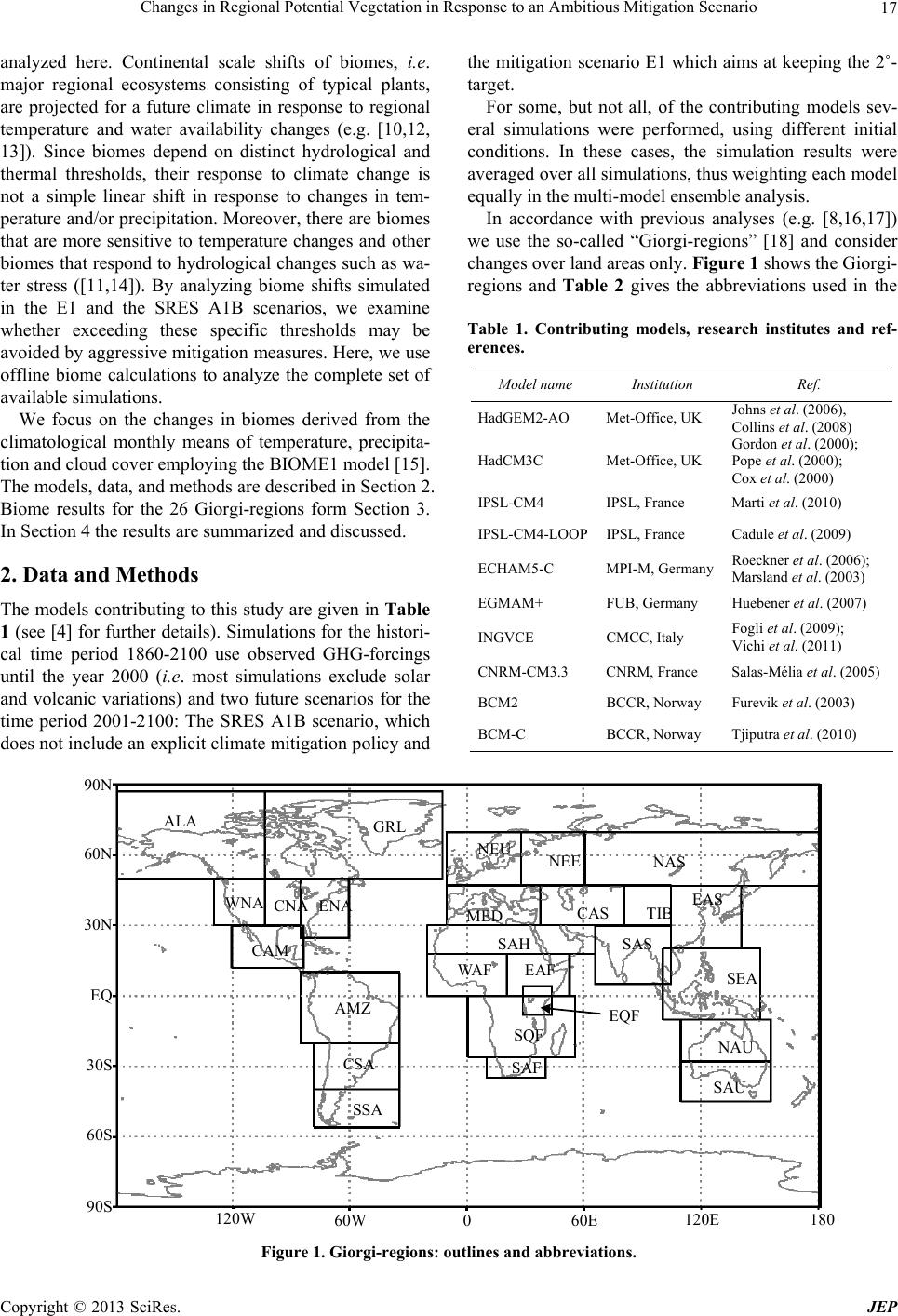

Changes in Regional Potential Vegetation in Response to an Ambitious Mitigation Scenario 17

analyzed here. Continental scale shifts of biomes, i.e.

major regional ecosystems consisting of typical plants,

are projected for a future climate in response to regional

temperature and water availability changes (e.g. [10,12,

13]). Since biomes depend on distinct hydrological and

thermal thresholds, their response to climate change is

not a simple linear shift in response to changes in tem-

perature and/or precipitation. Moreover, there are biomes

that are more sensitive to temperature changes and other

biomes that respond to hydrological changes such as wa-

ter stress ([11,14]). By analyzing biome shifts simulated

in the E1 and the SRES A1B scenarios, we examine

whether exceeding these specific thresholds may be

avoided by aggressive mitigation measures. Here, we use

offline biome calculations to analyze the complete set of

available simulations.

We focus on the changes in biomes derived from the

climatological monthly means of temperature, precipita-

tion and cloud cover employing the BIOME1 model [15].

The models, data, and methods are described in Section 2.

Biome results for the 26 Giorgi-regions form Section 3.

In Section 4 the results are summarized and discussed.

2. Data and Methods

The models contributing to this study are given in Table

1 (see [4] for further details). Simulations for the histori-

cal time period 1860-2100 use observed GHG-forcings

until the year 2000 (i.e . most simulations exclude solar

and volcanic variations) and two future scenarios for the

time period 2001-2100: The SRES A1B scenario, which

does not include an explicit climate mitigation policy and

the mitigation scenario E1 which aims at keeping the 2˚-

target.

For some, but not all, of the contributing models sev-

eral simulations were performed, using different initial

conditions. In these cases, the simulation results were

averaged over all simulations, thus weighting each model

equally in the multi-model ensemble analysis.

In accordance with previous analyses (e.g. [8,16,17])

we use the so-called “Giorgi-regions” [18] and consider

changes over land areas only. Figure 1 shows the Giorgi-

regions and Table 2 gives the abbreviations used in the

Table 1. Contributing models, research institutes and ref-

erences.

Model name Institution Ref.

HadGEM2-AO Met-Office, UK

Johns et al. (2006),

Collins et al. (2008)

HadCM3C Met-Office, UK

Gordon et al. (2000);

Pope et al. (2000);

Cox et al. (2000)

IPSL-CM4 IPSL, France Marti et al. (2010)

IPSL-CM4-LOOPIPSL, France Cadule et al. (2009)

ECHAM5-C MPI-M, Germany

Roeckner et al. (2006);

Marsland et al. (2003)

EGMAM+ FUB, Germany Huebener et al. (2007)

INGVCE CMCC, Italy

Fogli et al. (2009);

Vichi et al. (2011)

CNRM-CM3.3 CNRM, France Salas-Mélia et al. (2005)

BCM2 BCCR, Norway Furevik et al. (2003)

BCM-C BCCR, Norway Tjiputra et al. (2010)

ALA GRL

WNA CNA ENA

CAM

AMZ

CSA

SSA

NEU NEE NAS

MED CAS TIB

EAS

SAS

SEA

NAU

SAH

WAF EAF

EQF

SQF

SAF

120W 60W 60E 0 120E 180

90S

60S

30S

30N

60N

90N

Figure 1. Giorgi-regions: outlines and abbreviations.

C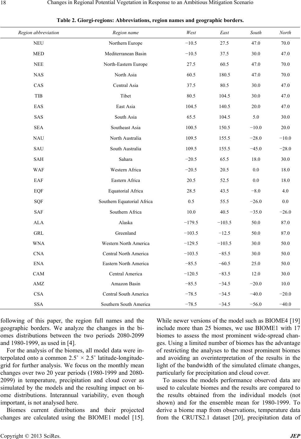hanges in Regional Potential Vegetation in Response to an Ambitious Mitigation Scenario

Table 2. Giorgi-regions: Abbreviations, region names and geographic borders.

Region abbreviation Region name West East South North

NEU Northern Europe −10.5 27.5 47.0 70.0

MED Mediterranean Basin −10.5 37.5 30.0 47.0

NEE North-Eastern Europe 27.5 60.5 47.0 70.0

NAS North Asia 60.5 180.5 47.0 70.0

CAS Central Asia 37.5 80.5 30.0 47.0

TIB Tibet 80.5 104.5 30.0 47.0

EAS East Asia 104.5 140.5 20.0 47.0

SAS South Asia 65.5 104.5 5.0 30.0

SEA Southeast Asia 100.5 150.5 −10.0 20.0

NAU North Australia 109.5 155.5 −28.0 −10.0

SAU South Australia 109.5 155.5 −45.0 −28.0

SAH Sahara −20.5 65.5 18.0 30.0

WAF Western Africa −20.5 20.5 0.0 18.0

EAF Eastern Africa 20.5 52.5 0.0 18.0

EQF Equatorial Africa 28.5 43.5 −8.0 4.0

SQF Southern Equatorial Africa 0.5 55.5 −26.0 0.0

SAF Southern Africa 10.0 40.5 −35.0 −26.0

ALA Alaska −179.5 −103.5 50.0 87.0

GRL Greenland −103.5 −12.5 50.0 87.0

WNA Western North America −129.5 −103.5 30.0 50.0

CNA Central North America −103.5 −85.5 30.0 50.0

ENA Eastern North America −85.5 −60.5 25.0 50.0

CAM Central America −120.5 −83.5 12.0 30.0

AMZ Amazon Basin

−85.5 −34.5 −20.0 10.0

CSA Central South America −78.5 −34.5 −40.0 −20.0

SSA Southern South America −78.5 −34.5 −56.0 −40.0

following of this paper, the region full names and the

geographic borders. We analyze the changes in the bi-

omes distributions between the two periods 2080-2099

and 1980-1999, as used in [4].

For the analysis of the biomes, all model data were in-

terpolated onto a common 2.5˚ × 2.5˚ latitude-longitude-

grid for further analysis. We focus on the monthly mean

changes over two 20 year periods (1980-1999 and 2080-

2099) in temperature, precipitation and cloud cover as

simulated by the models and the resulting impact on bi-

ome distributions. Interannual variability, even though

important, is not analysed here.

Biomes current distributions and their projected

changes are calculated using the BIOME1 model [15].

While newer versions of the model such as BIOME4 [19]

include more than 25 biomes, we use BIOME1 with 17

biomes to assess the most prominent wide-spread chan-

ges. Using a limited number of biomes has the advantage

of restricting the analyses to the most prominent biomes

and avoiding an overinterpretation of the results in the

light of the bandwidth of the simulated climate changes,

particularly for precipitation and cloud cover.

To assess the models performance observed data are

used to calculate biomes and the results are compared to

the results obtained from the individual models (not

shown) and for the ensemble mean for 1980-1999. To

derive a biome map from observations, temperature data

from the CRUTS2.1 dataset [20], precipitation data of

C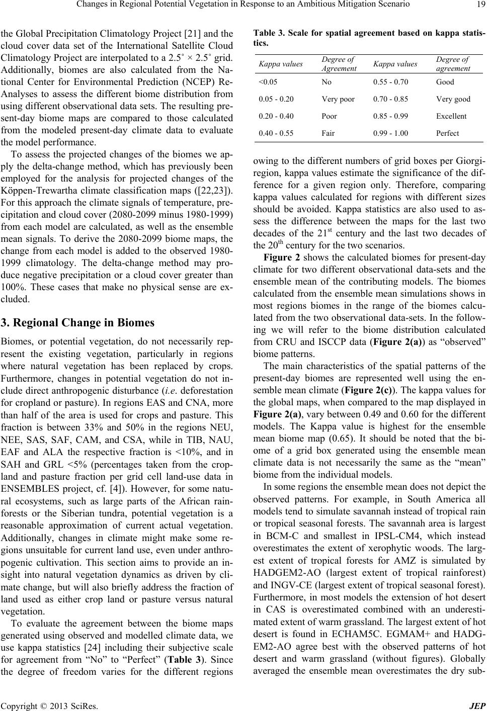hanges in Regional Potential Vegetation in Response to an Ambitious Mitigation Scenario 19

the Global Precipitation Climatology Project [21] and the

cloud cover data set of the International Satellite Cloud

Climatology Project are interpolated to a 2.5˚ × 2.5˚ grid.

Additionally, biomes are also calculated from the Na-

tional Center for Environmental Prediction (NCEP) Re-

Analyses to assess the different biome distribution from

using different observational data sets. The resulting pre-

sent-day biome maps are compared to those calculated

from the modeled present-day climate data to evaluate

the model performance.

To assess the projected changes of the biomes we ap-

ply the delta-change method, which has previously been

employed for the analysis for projected changes of the

Köppen-Trewartha climate classification maps ([22,23]).

For this approach the climate signals of temperature, pre-

cipitation and cloud cover (2080-2099 minus 1980-1999)

from each model are calculated, as well as the ensemble

mean signals. To derive the 2080-2099 biome maps, the

change from each model is added to the observed 1980-

1999 climatology. The delta-change method may pro-

duce negative precipitation or a cloud cover greater than

100%. These cases that make no physical sense are ex-

cluded.

3. Regional Change in Biomes

Biomes, or potential vegetation, do not necessarily rep-

resent the existing vegetation, particularly in regions

where natural vegetation has been replaced by crops.

Furthermore, changes in potential vegetation do not in-

clude direct anthropogenic disturbance (i.e. deforestation

for cropland or pasture). In regions EAS and CNA, more

than half of the area is used for crops and pasture. This

fraction is between 33% and 50% in the regions NEU,

NEE, SAS, SAF, CAM, and CSA, while in TIB, NAU,

EAF and ALA the respective fraction is <10%, and in

SAH and GRL <5% (percentages taken from the crop-

land and pasture fraction per grid cell land-use data in

ENSEMBLES project, cf. [4]). However, for some natu-

ral ecosystems, such as large parts of the African rain-

forests or the Siberian tundra, potential vegetation is a

reasonable approximation of current actual vegetation.

Additionally, changes in climate might make some re-

gions unsuitable for current land use, even under anthro-

pogenic cultivation. This section aims to provide an in-

sight into natural vegetation dynamics as driven by cli-

mate change, but will also briefly address the fraction of

land used as either crop land or pasture versus natural

vegetation.

To evaluate the agreement between the biome maps

generated using observed and modelled climate data, we

use kappa statistics [24] including their subjective scale

for agreement from “No” to “Perfect” (Table 3). Since

the degree of freedom varies for the different regions

Table 3. Scale for spatial agreement based on kappa statis-

tics.

Kappa values Degree of

Agreement Kappa values Degree of

agreement

<0.05 No 0.55 - 0.70 Good

0.05 - 0.20 Very poor 0.70 - 0.85 Very good

0.20 - 0.40 Poor 0.85 - 0.99 Excellent

0.40 - 0.55 Fair 0.99 - 1.00 Perfect

owing to the different numbers of grid boxes per Giorgi-

region, kappa values estimate the significance of the dif-

ference for a given region only. Therefore, comparing

kappa values calculated for regions with different sizes

should be avoided. Kappa statistics are also used to as-

sess the difference between the maps for the last two

decades of the 21st century and the last two decades of

the 20th century for the two scenarios.

Figure 2 shows the calculated biomes for present-day

climate for two different observational data-sets and the

ensemble mean of the contributing models. The biomes

calculated from the ensemble mean simulations shows in

most regions biomes in the range of the biomes calcu-

lated from the two observational data-sets. In the follow-

ing we will refer to the biome distribution calculated

from CRU and ISCCP data (Figure 2(a)) as “observed”

biome patterns.

The main characteristics of the spatial patterns of the

present-day biomes are represented well using the en-

semble mean climate (Figure 2(c)). The kappa values for

the global maps, when compared to the map displayed in

Figure 2(a), vary between 0.49 and 0.60 for the different

models. The Kappa value is highest for the ensemble

mean biome map (0.65). It should be noted that the bi-

ome of a grid box generated using the ensemble mean

climate data is not necessarily the same as the “mean”

biome from the individual models.

In some regions the ensemble mean does not depict the

observed patterns. For example, in South America all

models tend to simulate savannah instead of tropical rain

or tropical seasonal forests. The savannah area is largest

in BCM-C and smallest in IPSL-CM4, which instead

overestimates the extent of xerophytic woods. The larg-

est extent of tropical forests for AMZ is simulated by

HADGEM2-AO (largest extent of tropical rainforest)

and INGV-CE (largest extent of tropical seasonal forest).

Furthermore, in most models the extension of hot desert

in CAS is overestimated combined with an underesti-

mated extent of warm grassland. The largest extent of hot

desert is found in ECHAM5C. EGMAM+ and HADG-

EM2-AO agree best with the observed patterns of hot

desert and warm grassland (without figures). Globally

averaged the ensemble mean ates the dry sub- overestim

C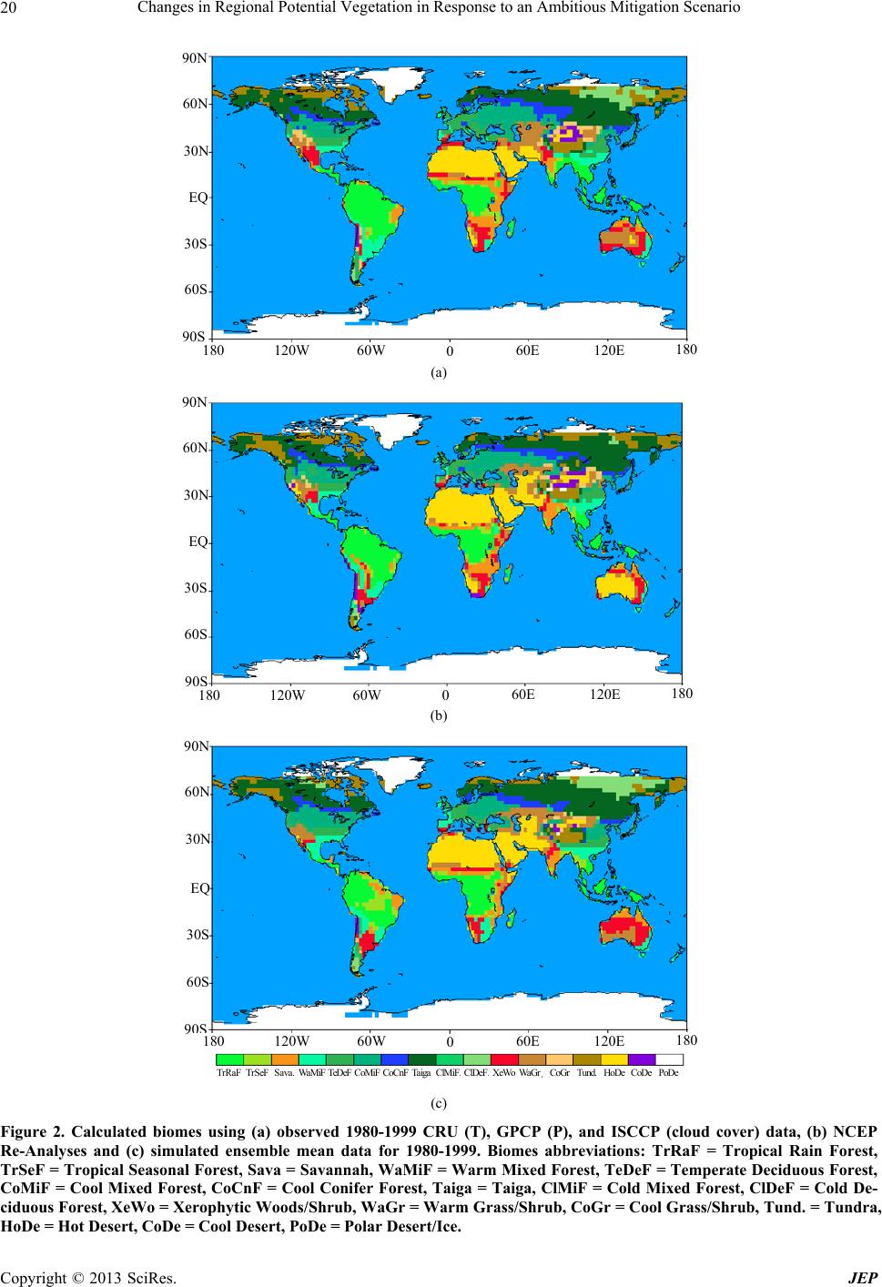hanges in Regional Potential Vegetation in Response to an Ambitious Mitigation Scenario

120W 60W60E

0120E 180

90S

60S

30S

30N

60N

90N

180

(a)

120W 60W 60E

120E 180

90S

60S

30S

30N

60N

90N

180

(b)

120W 60W60E

0120E 18

90S

60S

30S

30N

60N

90N

180

TrRaF TrSeF Sava. Wa M i F TeDeF CoMiFCoCnFTaiga ClMiF ClDeF XeWoWaGr CoGr Tund. HoDe CoDe PoDe

(c)

Figure 2. Calculated biomes using (a) observed 1980-1999 CRU (T), GPCP (P), and ISCCP (cloud cover) data, (b) NCEP

Re-Analyses and (c) simulated ensemble mean data for 1980-1999. Biomes abbreviations: TrRaF = Tropical Rain Forest,

TrSeF = Tropical Seasonal Forest, Sava = Savannah, WaMiF = Warm Mixed Forest, TeDeF = Temperate Deciduous Forest,

CoMiF = Cool Mixed Forest, CoCnF = Cool Conifer Forest, Taiga = Taiga, ClMiF = Cold Mixed Forest, ClDeF = Cold De-

ciduous Forest, XeWo = Xerophytic Woods/Shrub, WaGr = Warm Grass/Shrub, CoGr = Cool Grass/Shrub, Tund. = Tundra,

HoDe = Hot Desert, CoDe = Cool Desert, PoDe = Polar Desert/Ice.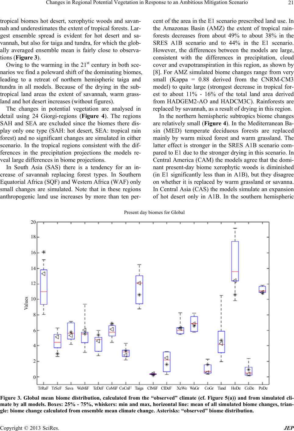

Changes in Regional Potential Vegetation in Response to an Ambitious Mitigation Scenario 21

tropical biomes hot desert, xerophytic woods and savan-

nah and underestimates the extent of tropical forests. Lar-

gest ensemble spread is evident for hot desert and sa-

vannah, but also for taiga and tundra, for which the glob-

ally averaged ensemble mean is fairly close to observa-

tions (Figure 3).

Owing to the warming in the 21st century in both sce-

narios we find a poleward shift of the dominating biomes,

leading to a retreat of northern hemispheric taiga and

tundra in all models. Because of the drying in the sub-

tropical land areas the extent of savannah, warm grass-

land and hot desert increases (without figures).

The changes in potential vegetation are analysed in

detail using 24 Giorgi-regions (Figure 4). The regions

SAH and SEA are excluded since the biomes there dis-

play only one type (SAH: hot desert, SEA: tropical rain

forest) and no significant changes are simulated in either

scenario. In the tropical regions consistent with the dif-

ferences in the precipitation projections the models re-

veal large differences in biome projections.

In South Asia (SAS) there is a tendency for an in-

crease of savannah replacing forest types. In Southern

Equatorial Africa (SQF) and Western Africa (WAF) only

small changes are simulated. Note that in these regions

anthropogenic land use increases by more than ten per-

cent of the area in the E1 scenario prescribed land use. In

the Amazonas Basin (AMZ) the extent of tropical rain-

forests decreases from about 49% to about 38% in the

SRES A1B scenario and to 44% in the E1 scenario.

However, the differences between the models are large,

consistent with the differences in precipitation, cloud

cover and evapotranspiration in this region, as shown by

[8]. For AMZ simulated biome changes range from very

small (Kappa = 0.88 derived from the CNRM-CM3

model) to quite large (strongest decrease in tropical for-

est to about 11% - 16% of the total land area derived

from HADGEM2-AO and HADCM3C). Rainforests are

replaced by savannah, as a result of drying in this region.

In the northern hemispheric subtropics biome changes

are relatively small (Figure 4). In the Mediterranean Ba-

sin (MED) temperate deciduous forests are replaced

mainly by warm mixed forest and warm grassland. The

latter effect is stronger in the SRES A1B scenario com-

pared to E1 due to the stronger drying in this scenario. In

Central America (CAM) the models agree that the domi-

nant present-day biome xerophytic woods is diminished

(in E1 significantly less than in A1B), but they disagree

on whether it is replaced by warm grassland or savanna.

In Central Asia (CAS) the models simulate an expansion

of hot desert only in A1B. In the southern hemispheric

TrRaF TrSeF Sava Wa M iF TeDe F CoMiFCoCnFTaiga ClMiF ClDeF XeWoWaGr CoGr Tund HoDe CoDe PoDe

Va lues

Present day biomes for Global

Figure 3. Global mean biome distribution, calculated from the “observed” climate (cf. Figure 5(a)) and from simulated cli-

mate by all models. Boxes: 25% - 75%, whiskers: min and max, horizontal line: mean of all simulated biome changes, trian-

gle: biome change calculated from ensemble mean climate change. Asterisks: “observed” biome distribution.

C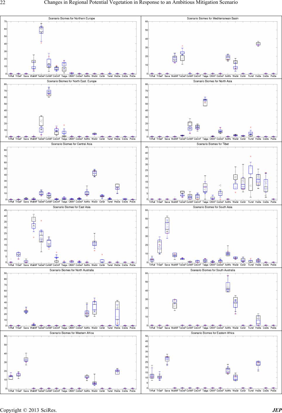hanges in Regional Potential Vegetation in Response to an Ambitious Mitigation Scenario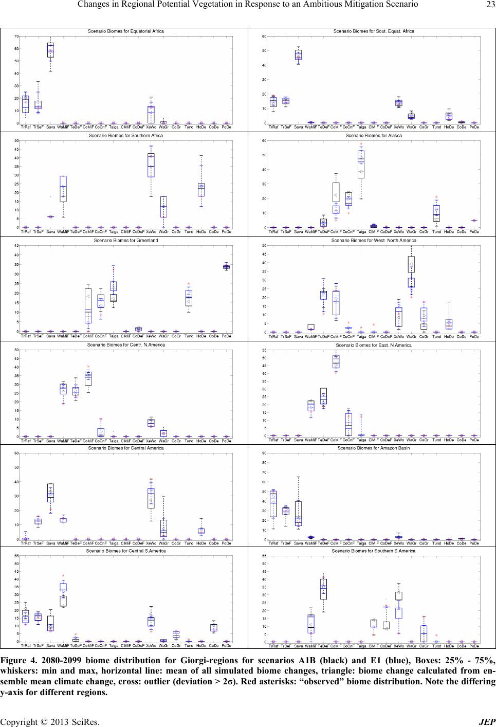

Changes in Regional Potential Vegetation in Response to an Ambitious Mitigation Scenario 23

Figure 4. 2080-2099 biome distribution for Giorgi-regions for scenarios A1B (black) and E1 (blue), Boxes: 25% - 75%,

whiskers: min and max, horizontal line: mean of all simulated biome changes, triangle: biome change calculated from en-

semble mean climate change, cross: outlier (deviation > 2σ). Red asterisks: “observed” biome distribution. Note the differing

-axis for different regions. y

C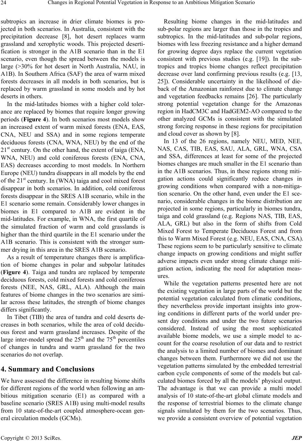hanges in Regional Potential Vegetation in Response to an Ambitious Mitigation Scenario

subtropics an increase in drier climate biomes is pro-

jected in both scenarios. In Australia, consistent with the

precipitation decrease [8], hot desert replaces warm

grassland and xerophytic woods. This projected deserti-

fication is stronger in the A1B scenario than in the E1

scenario, even though the spread between the models is

large (>30% for hot desert in North Australia, NAU, in

A1B). In Southern Africa (SAF) the area of warm mixed

forests decreases in all models in both scenarios, but is

replaced by warm grassland in some models and by hot

deserts in others.

In the mid-latitudes biomes with a higher cold toler-

ance are replaced by biomes that require longer growing

periods (Figure 4). In both scenarios most models show

an increased extent of warm mixed forests (ENA, EAS,

CNA, NEU and SSA) and in some regions temperate

deciduous forests (CNA, WNA, NEU) by the end of the

21st century. On the other hand, the extent of taiga (ENA,

WNA, NEU) and cold coniferous forests (ENA, CNA,

EAS) decreases according to most models. In Northern

Europe (NEU) tundra disappears in all models by the end

of the 21st century. In (WNA) taiga and cool mixed forest

disappear in both scenarios. In addition, cold coniferous

forests disappear in the SRES A1B scenario, while in the

E1 scenario some remain. Considerably lower changes in

biomes in E1 compared to A1B are evident in the

mid-latitudes. For example, in WNA, the first quartile of

the simulated fraction of warm and cold grasslands is

higher than the third quartile in the E1 scenario under the

A1B scenario. This is consistent with the stronger sum-

mer drying in this area in the SRES A1B scenario.

As a result of temperature changes there is amplifica-

tion of biome changes in polar and subpolar latitudes

(Figure 4). Taiga and tundra are replaced by temperate

deciduous forests, cold mixed forests and cold coniferous

forests (NEE, NAS, GRL, ALA). Although the main

features of biome changes in the two scenarios are simi-

lar across these latitudes, the strength of biome changes

differs significantly.

In Tibet (TIB) the area of tundra and cold deserts de-

creases in both scenarios, while the area of cold decidu-

ous forest and warm grassland increases. Despite of the

large inter-model spread the 25th and the 75th percentiles

of changes in tundra and warm grassland for the two

scenarios do not overlap.

4. Summary and Conclusions

We have assessed the difference in resulting biome shifts

for different regions of the world when following an am-

bitious mitigation scenario (E1) as compared with a

baseline scenario (SRES A1B) using multi-model results

from 10 state-of-the-art coupled atmosphere-ocean gen-

eral circulation models (GCMs).

Resulting biome changes in the mid-latitudes and

sub-polar regions are larger than those in the tropics and

subtropics. In the mid-latitudes and sub-polar regions,

biomes with less freezing resistance and a higher demand

for growing degree days replace the current vegetation

consistent with previous studies (e.g. [19]). In the sub-

tropics and tropics biome changes reflect precipitation

decrease over land confirming previous results (e.g. [13,

25]). Considerable uncertainty in the likelihood of die-

back of the Amazonian rainforest due to climate change

and vegetation feedbacks remains [26]. The particularly

strong potential vegetation change for the Amazonas

region in HadCM3C and HadGEM2-AO compared to the

other analyzed GCMs is consistent with the simulated

strong forcing response in these regions for precipitation

and cloud cover as shown by [8].

In 13 of the 26 regions, namely NEU, MED, NEE,

NAS, CAS, TIB, EAS, SAU, ALA, GRL, WNA, CSA

and SSA, differences at least for some of the projected

biomes changes are much smaller in the E1 scenario than

in the A1B scenarios. Thus, in these regions strong miti-

gation actions could significantly reduce changes in

growing conditions when compared with a non-mitiga-

tion scenario. On the other hand, even under the E1 sce-

nario, considerable changes in the biome distribution are

projected in some regions, particularly in biomes tundra,

taiga and cold grassland (e.g. Regions NAS, TIB, EAS,

ALA, GRL) but also in the form of shifts from Cold

Mixed Forest to Temperate Deciduous Forest and from

this to Warm Mixed Forest (e.g. NEU, EAS, CNA, CSA).

These regions seem to be particularly sensitive to climate

change impacts on growing conditions and might suffer

adverse impacts even under strong climate change miti-

gation action, indicating the need for adaptation meas-

ures.

While the vegetation patterns presented here are not

the existing vegetation in large parts of the world but the

potential vegetation calculated from climatic conditions,

they nevertheless provide important insights into grow-

ing conditions in different parts of the world under pre-

sent day conditions and under the two future scenarios

considered. Instead of using the most sophisticated

available biome models, we use a simple model to ac-

count for the coarse resolution of our data and to restrict

the analysis to a limited number of biomes and dominant

changes between them. Furthermore we did not use the

vegetation patterns simulated by the embedded terrestrial

carbon cycle components of some of the models but cal-

culated biomes forced by all the models’ physical output.

The advantage is that we can provide a multi model

analysis of 10 state-of-the-art global climate models and

the response of terrestrial biomes to the climate change

signals simulated by them for the two scenarios. Thus,

we provide a consistent overview of potential vegetation

Changes in Regional Potential Vegetation in Response to an Ambitious Mitigation Scenario 25

response to an ambitious mitigation scenario (E1) com-

pared to a baseline scenario (A1B). Further research

should focus on the regions with the largest sensitivity to

climate change with respect to growing conditions. In

these regions, both natural vegetation and anthropogenic

land-use should be reviewed as to their resilience under

projected climate change for different forcing scenarios.

5. Acknowledgements

The ENSEMBLES model-outputs used in this work were

produced with the partial funding of the EU FP6 Inte-

grated Project ENSEMBLES (Contract number 505539),

whose support is gratefully acknowledged.

REFERENCES

[1] R. H. Moss, et al., “The Next Generation of Scenarios for

Climate Change Research and Assessment,” Nature, Vol.

463, 2010, pp. 747-756. doi:10.1038/nature08823

[2] P. van der Linden and J. F. B. Mitchell, “ENSEMBLES:

Climate Change and Its Impacts: Summary of Research

and Results from the ENSEMBLES Project,” Met Office

Hadley Centre, 2009, 160 p.

[3] J. A. Lowe, C. D. Hewitt, D. P. van Vuuren, T. C. Johns,

E. Stehfest, J.-F. Royer and P. J. van der Linden, “New

Study for Climate Modeling, Analyses, and Scenarios,”

Eos, Transactions American Geophysical Union, Vol. 90,

No. 21, 2009, pp. 181-182.

doi:10.1029/2009EO210001

[4] T. C. Johns, J.-F. Royer, I. Höschel, H. Huebener, E.

Roeckner, E., Manzini, W. May, J.-L. Dufresne, O. H.

Otterå, D. P. van Vuuren, D. Salas y Melia, M. Giorgetta,

S. Denvil, S. Yang, P. G. Fogli, J. Körper and C. D. Hew-

itt, “Climate Change under Aggressive Mitigation: The

ENSEMBLES Multi-Model Experiment,” Climate Dy-

namics, Vol. 37, No. 9-10, 2011, pp. 1975-2003.

doi:10.1007/s00382-011-1005-5

[5] D. G. Streets, et al., “Two-Decadal Aerosol Trends as a

Likely Explanation of the Global Dimming/Brightening

Transition,” Geophysical Research Letters, Vol. 33, No.

15, 2006, p. L15806. doi:10.1029/2006GL026471

[6] M. I. Mischchenko, et al., “Long-Term Satellite Record

Reveals Likely Recent Aerosol Trend,” Science, Vol. 315,

No. 5851, 2007, p. 1543. doi:10.1126/science.1136709

[7] G. A. Meehl, T. F. Stocker, et al., “Global Climate Pro-

jections,” In: S. Solomon, et al., Eds., Climate Change

2007: The Physical Science Basis, Cambridge University

Press, Cambridge, New York, 2007, pp. 747-846.

[8] H. Huebener, M. G. Sanderson, I. Höschel, J. Körper, T.

C. Johns, J.-F. Royer, E. Roeckner, E. Manzini, J.-L. Du-

fresne, O. H. Otterå, J. Tjiputra, D. S. Y Melia, M. Gior-

getta, S. Denvil and P. G. Fogli, “Regional Hydrological

Cycle Changes in Response to an Ambitious Mitigation

Scenario,” Climatic Change, 2013.

doi:10.1007/s10584-013-0829-x

[9] J. Körper, I. Höschel, J. A. Lowe, C. D. Hewitt, D. Salas

y Melia, E. Roeckner, H. Huebener, J.-F. Royer, J.-L.

Dufresne, A. Pardaens, M. A. Giorgetta, M. G. Sanderson,

O. H. Otterå, J. Tjiputra and S. Denvil, “The Effects of

Aggressive Mitigation on Steric Sea Level Rise and Sea

Ice Changes,” Climate Dynamics, Vol. 40, No. 3-4, 2013,

pp. 531-550. doi:10.1007/s00382-012-1612-9

[10] A. Fischlin, G. F. Midgley, J. T. Price, R. Leemans, B.

Gopal, C. Turley, M. D. A. Rounsevell, O. P. Dube, J.

Tarazona and A. A. Velichko, “Ecosystems, Their Prop-

erties, Goods, and Services,” In: M. L. Parry, O. F. Can-

ziani, J. P. Palutikof, P. J. van der Linden and C. E. Han-

son, Eds., Climate Change 2007: Impacts, Adaptation and

Vulnerability, Cambridge University Press, Cambridge,

2007, pp. 211-272.

[11] O. E. Sala, F. S. Chapin, J. J. Armesto, E. Berlow, J.

Bloomfield, R. Dirzo, E. Huber-Sanwald, L. F. Huenneke,

R. B. Jackson, A. Kinzig, R. Leemans, D. M. Lodge, H.

A. Mooney, M. Oesterheld, A. L. Poff, M. T. Sykes, B. H.

Walker, M. Walker and D. H. Wall, “Global Biodiversity

Scenarios for the Year 2100,” Science, Vol. 287, No.

5459, 2000, pp. 1770-1774.

[12] A. D. Hansen, R. P. Neilson, V. H. Dale, C. H. Flather, L.

R. Iverson, D. J. Currie, S. Shaver, R. Cook and P. J.

Bartlein, “Global Change in Forests: Responses of Spe-

cies, Communities and Biomes,” BioScience, Vol. 51, No.

9, 2001, pp. 765-779.

doi:10.1641/0006-3568(2001)051[0765:GCIFRO]2.0.CO

[13] S. Sitch, C. Huntingford, N. Gedney, P. E. Levy, M. Lo-

mas, S. L. Piao, R. Betts, P. Ciais, P. Cox, P. Friedling-

stein, C. D. Jones, I. C. Prentice and F. I. Woodward,

“Evaluation of the Terrestrial Carbon Cycle, Future Plant

Geography and Climate-Carbon Cycle Feedbacks Using

Five Dynamic Global Vegetation Models (DGVMs),”

Global Change Biology, Vol. 14, No. 9, 2008, pp. 2015-

2039. doi:10.1111/j.1365-2486.2008.01626.x

[14] M. Kirschbaum and A. Fischlin, “Climate Change Im-

pacts on Forests,” In: R. Watson, M. C. Zinyowera and R.

H. Moss, Eds., Climate Change 1995: Impacts; Adapta-

tions and Mitigation of Climate Change. Scientific-Tech-

nical Analysis, Cambridge University Press, Cambridge,

1996, pp. 95-129.

[15] I. C. Prentice, W. Cramer, S. P. Harrison, R. Leemans, R.

A. Monserud and M. A. Solomon, “A Global Biome

Model Based on Plant Physiology and Dominance, Soil

Properties and Climate” Journal of Biogeography, Vol.

19, No. 2, 1992, pp. 117-134. doi:10.2307/2845499

[16] W. May, “Climatic Changes Associated with a Global

‘2˚C-Stabilization’ Scenario Simulated by the ECHAM5/

MPI-OM Coupled Climate Model,” Climate Dynamics,

Vol. 31, No. 2-3, 2008, pp. 283-313.

doi:10.1007/s00382-007-0352-8

[17] J. H. Christensen, B. Hewitson, et al., “Regional Climate

Projections,” In: S. Solomon, et al., Eds., Climate Change

2007: The Physical Science Basis, Cambridge University

Press, Cambridge, New York, 2007, Chapter 11.

[18] F. Giorgi and X. Bi, “Updated Regional Precipitation and

Temperature Changes for the 21st Century from Ensem-

bles of Recent AOGCM Simulations,” Geophysical Re-

search Letters, Vol. 32, No. 21, 2005, p. L21715.

doi:10.1029/2005GL024288

Changes in Regional Potential Vegetation in Response to an Ambitious Mitigation Scenario

[19] J. O. Kaplan, et al., “Climate Change and Arctic Ecosys-

tems: 2. Modeling, Paleodata-Model Comparisons, and

Future Projections,” Journal of Geophysical Research:

Atmospheres, Vol. 108, No. D19, 2003, p. 8171.

doi:10.1029/2002JD002559

[20] T. D. Mitchell and P. D. Jones, “An Improved Method of

Constructing a Database of Monthly Climate Observa-

tions and Associated High-Resolution Grids,” Journal of

Geophysical Research: Atmospheres, Vol. 25, No. 6,

2005, pp. 693-712. doi:10.1002/joc.1181

[21] G. J. Huffman, R. F. Adler, M. Morrissey, D. T. Bolvin, S.

Curtis, R. Joyce, B. McGavock and J. Susskind, “Global

Precipitation at One-Degree Daily Resolution from Multi-

Satellite Observations,” Journal of Hydrometeorology,

Vol. 2, No. 1, 2001, pp. 36-50.

doi:10.1175/1525-7541(2001)002<0036:GPAODD>2.0.C

O;2

[22] M. de Castro, C. Gallardo, K. Jylha and K. Tuomenvirta,

“The Use of a Climate-Type Classification for Assessing

Climate Change Effects in Europe from Ensemble of

Nine Regional Climate Models,” Climatic Change, Vol.

81, No. 1, 2007, pp. 329-342.

doi:10.1007/s10584-006-9224-1

[23] F. Hanf, J. Körper, T. Spangehl and U. Cubasch, “Shifts

of Climate Zones in Multi-Model Climate Change Expe-

riments Using the Koppen Climate Classification,” Mete-

orologische Zeitschrift, Vol. 21, No. 2, 2012, pp. 111-123.

doi:10.1127/0941-2948/2012/0344

[24] R. A. Monserud and R. Leemans, “Comparing Global

Vegetation Maps with the Kappa Statistic,” Ecological

Modelling, Vol. 62, No. 4, 1992, pp. 275-293.

doi:10.1016/0304-3800(92)90003-W

[25] C. A. Alo and G. Wang, “Potential Future Changes of the

Terrestrial Ecosystem Based on Climate Projections by

Eight General Circulation Models,” Journal of Geophy-

sical Research, Vol. 113, No. G1, 2008, p. G01004.

doi:10.1029/2007JG000528

[26] Y. Malhi, et al., “Exploring the Likelihood and Mecha-

nism of a Climate-Change Induced Dieback of the Ama-

zon Rainforest,” Proceedings of the National Academy of

Sciences, Vol. 106, No. 49, 2009, pp. 20610-20615.

doi:10.1073/pnas.0804619106