How soon would the next mega-earthquake occur in Japan?

doi:10.4236/ns.2013.58A1001

Paper Menu >>

Journal Menu >>

Vol.5, No.8A1, 1-7 (2013) Natural Science

http://dx.doi.org/10.4236/ns.2013.58A1001

How soon would the next mega-earthquake

occur in Japan?

Alexey Lyu bushin

Institute of Physics of the Earth, Russian Academy of Sciences, Moscow, Russia; [email protected]

Received 12 May 2013; revised 12 July 2013; accepted 19 July 2013

which permits unrestricted use, distribution, and reproduction in any medium, provided the original work is properly cited.

ABSTRACT

The problem of seismic danger estimate in Ja-

pan after Tohoku mega-earthquake 11 March of

2011 is considered. The estimates are based on

processing low-frequency seismic noise wave-

forms from broadband network F-net. A new

method of dynamic estimate of seismic danger

is used for this problem. The method is based

on calculating multi-fractal properties and mini-

mum entropy of squared orthogonal wavelet

coefficients for seismic noise. The analysis of

the data using notion of “spots of seismic dan-

ger” shows that the seismic danger in Japan

remains at high level after 2011. 03. 11 within

north-east part of Philippine plate—at the region

of Nankai Though which traditionally is regarded

as the place of strongest earthquakes. It is well

known that estimate of time moment of future

shock is the most difficult problem in earth-

quake prediction. In this paper we try to find

some peculiarities of the seismic noise data

which could extract future danger time interval

by analogy with the behavior before Tohoku

earthquake. Two possible precursors of this

type were found. They are the results of esti-

mates within 1-year moving time window: based

on correlation between 2 mean multi-fractal pa-

rameters of the noise and based on cluster

analysis of annual clouds of 4 mean noise pa-

rameters. Both peculiarities of the noise data

extract time interval 2013-2014 as t he danger.

Keywords: Seismic Noise; Multi-Fractal Analysis;

Wavelet-Based Minimum Normalized Entropy;

Cluster Analysis; Earthquake Prediction; Dynamic

Estimate of Seismic Danger

1. INTRODUCTION

The problem of predicting strongest earthquakes in

Japan at the region of Nankai Trough is a traditional

large problem for seismologists in Japan [1,2]. In [1] the

probability of earthquake with magnitude more than 8.5

at Tokai-Nankai zone, the region where Philippine Sea

plate is approaching Central Japan, was estimated as 0.35

- 0.45 “for a ten-year period following the year 2000”. In

[3] the seismic danger for Japan was estimated immedi-

ately after Tohoku earthquake based on the analysis of

GPS data and the conclusion was that “estimates …

suggest the need to consider the potential for a future

large earthquake just south of this event.” In the paper [4]

the problem why the Tohoku earthquake was a surprise

for scientific community is discussed . One of the conclu-

sions in [4] is “A magnitude 9 earthquake off Tohoku

should not have been a surprise”. This conclusion was

made by retrospective analysis of seismic catalogs. Nev-

ertheless the Tohoku event was a great surprise for all

traditional methods of earthquake prediction. Other con-

clusion in [4] is that even magnitude 10 is quite po ssible

for Japan Trench.

Broadband seismic networks provide other type of in-

formation which could be used for earthquake prediction

as well. Low-frequency microseismic oscillations and

their correlation with the processes occurring in the hy-

drosphere and atmosphere of the Earth were investigated

in [5-7].

In papers [8-12] an analysis of the multi-fractal pa-

rameters of low-frequency seismic noise from the net-

work F-net provided a hypothesis that Japanese Islands

were approaching a large seismic catastrophe, the signa-

ture of which was a statistically significant decrease in

the support width of the multi-fractal singularity spec-

trum. A cluster analysis of background parameters led us

to conclude that in the middle of 2010 the islands of Ja-

pan entered a critically dangerous developmental phase

of seismic process [11] (the paper [11] was submitted at

April of 2010). The prediction of the catastrophe, first in

terms of approximate magnitude (middle of 2008) and

then in terms of approximate time (middle of 201 0), was

documented in advance in a series of papers and in pro-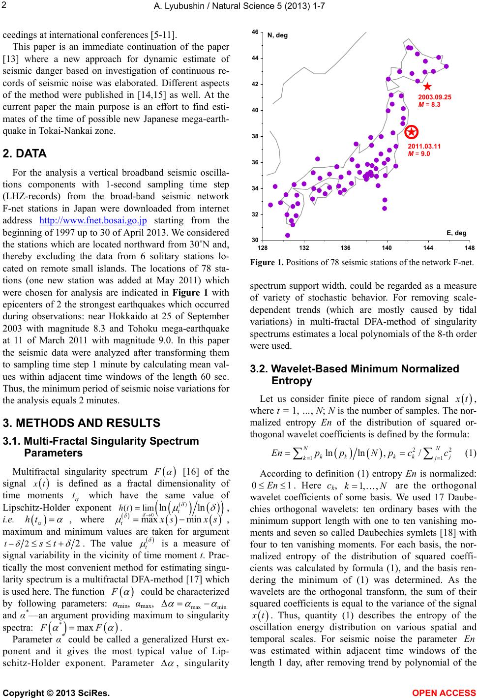

A. Lyubushin / Natural Science 5 (2013) 1-7

ceedings at international conferences [5-11].

This paper is an immediate continuation of the paper

[13] where a new approach for dynamic estimate of

seismic danger based on investigation of continuous re-

cords of seismic noise was elaborated. Different aspects

of the method were published in [14,15] as well. At the

current paper the main purpose is an effort to find esti-

mates of the time of possible new Japanese mega-earth-

quake in Tokai-Nankai zone.

2. DATA

For the analysis a vertical broadband seismic oscilla-

tions components with 1-second sampling time step

(LHZ-records) from the broad-band seismic network

F-net stations in Japan were downloaded from internet

address http://www.fnet.bosai.go.jp starting from the

beginning o f 19 97 up to 30 of A pr il 2 013. We cons ider ed

the stations which are located northward from 30˚N and,

thereby excluding the data from 6 solitary stations lo-

cated on remote small islands. The locations of 78 sta-

tions (one new station was added at May 2011) which

were chosen for analysis are indicated in Figure 1 with

epicenters of 2 the strongest earthquakes which occurred

during observations: near Hokkaido at 25 of September

2003 with magnitude 8.3 and Tohoku mega-earthquake

at 11 of March 2011 with magnitude 9.0. In this paper

the seismic data were analyzed after transforming them

to sampling time step 1 minute by calculating mean val-

ues within adjacent time windows of the length 60 sec.

Thus, the minimum period of seismic noise variations for

the analysis equals 2 minutes.

3. METHODS AND RESULTS

3.1. Multi-Fractal Singularity Spectrum

Parameters

Multifractal singularity spectrum





[16] of the

signal





t is defined as a fractal dimensionality of

time moments t



which have the same value of

Lipschitz-Holder exponent



mln t

()

() liln









,

i.e.





, where



ma min







s ,

maximum and minimum values are taken for argument

22t



 . The value t







is a measure of

signal variability in the vicinity of time moment t. Prac-

tically the most convenient method for estimating singu-

larity spectrum is a multifractal DFA-method [17] which

is used here. The function







could be characterized

by following parameters: αmin, αma x, max min











and α*—an argument providing maximum to singularity

spectra:





maxFF



.

Parameter α* could be called a generalized Hurst ex-

ponent and it gives the most typical value of Lip-

schitz-Holder exponent. Parameter



, singularity

128 132 136 140 144 148

N, deg

E, deg

2003.09.25

8.3

2011.03.11

9.0

Figure 1. Positions of 78 seismic stations of the network F-net.

spectrum support width, could be regarded as a measure

of variety of stochastic behavior. For removing scale-

dependent trends (which are mostly caused by tidal

variations) in multi-fractal DFA-method of singularity

spectrums estimates a local polynomials of the 8-th order

were used.

3.2. Wavelet-Based Minimum Normalized

Entropy

Let us consider finite piece of random signal





where t = 1, …, N; N is the number of samples. The nor-

malized entropy En of the distribution of squared or-

thogonal wavelet coefficients is defined by the formula:



lnln ,/

kk kk

EnppN pcc





(1)

According to definition (1) entropy En is normalized:

0En



. Here ck, 1, ,kN



 are the orthogonal

wavelet coefficients of some basis. We used 17 Daube-

chies orthogonal wavelets: ten ordinary bases with the

minimum support length with one to ten vanishing mo-

ments and seven so called Daubechies symlets [18] with

four to ten vanishing moments. For each basis, the nor-

malized entropy of the distribution of squared coeffi-

cients was calculated by formula (1), and the basis ren-

dering the minimum of (1) was determined. As the

wavelets are the orthogonal transform, the sum of their

squared coefficients is equal to the variance of the signal





t. Thus, quantity (1) describes the entropy of the

oscillation energy distribution on various spatial and

temporal scales. For seismic noise the parameter

was estimated within adjacent time windows of the

length 1 day, after removing trend by polynomial of the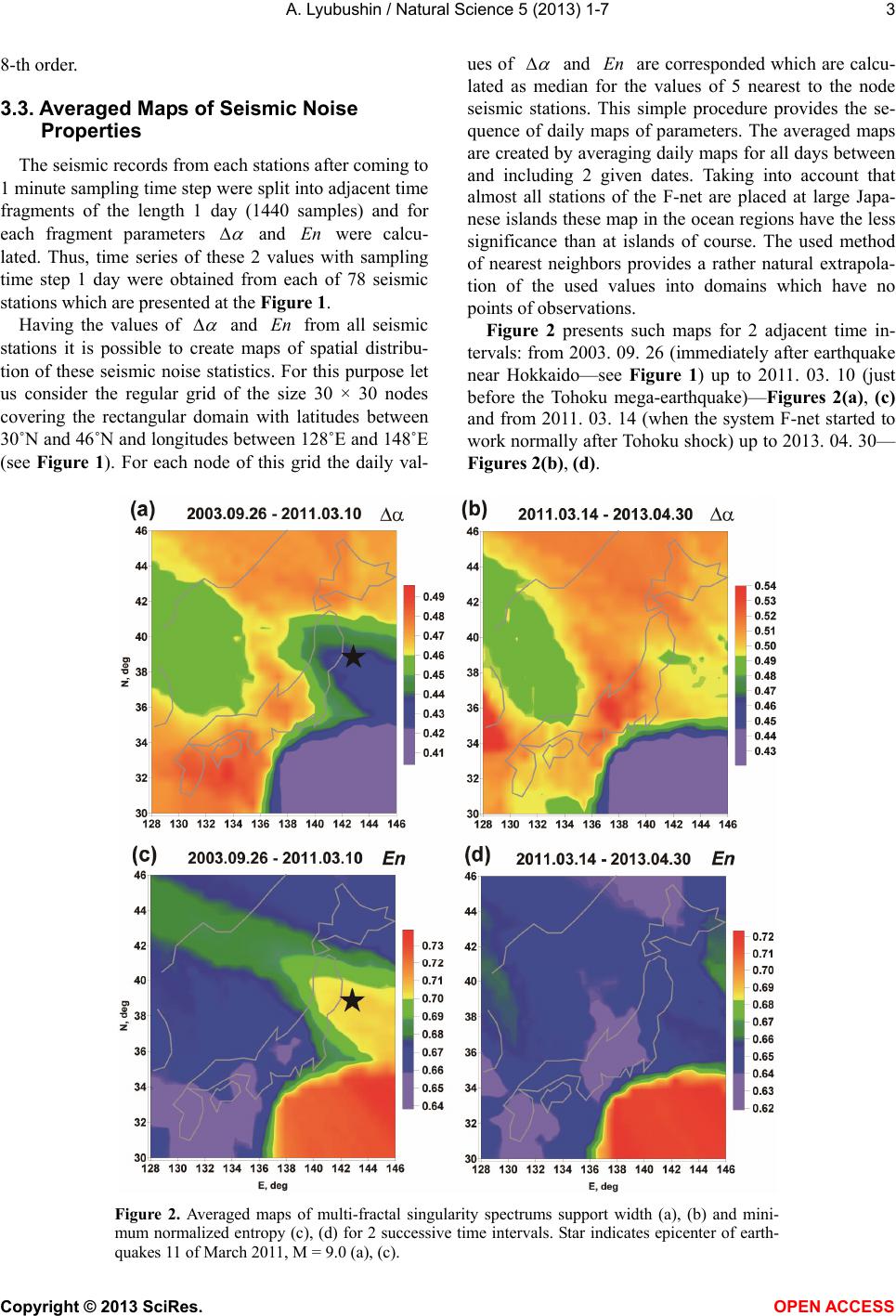

A. Lyubushin / Natural Science 5 (2013) 1-7

ues of





and are corresponded which are calcu-

lated as median for the values of 5 nearest to the node

seismic stations. This simple procedure provides the se-

quence of daily maps of parameters. The averaged maps

are created by averaging daily maps for all days between

and including 2 given dates. Taking into account that

almost all stations of the F-net are placed at large Japa-

nese islands these map in the ocean regions have the less

significance than at islands of course. The used method

of nearest neighbors provides a rather natural extrapola-

tion of the used values into domains which have no

points of observations.

8-th order.

3.3. Averaged Maps of Seismic Noise

Properties

The seismic records from each stations after coming to

1 minute sampling time step were split into adjacent time

fragments of the length 1 day (1440 samples) and for

each fragment parameters





and were calcu-

lated. Thus, time series of these 2 values with sampling

time step 1 day were obtained from each of 78 seismic

stations which are presented at the Figure 1.

Having the values of



 and from all seismic

stations it is possible to create maps of spatial distribu-

tion of these seismic noise statistics. For this purpose let

us consider the regular grid of the size 30 × 30 nodes

covering the rectangular domain with latitudes between

30˚N and 46˚N and longitudes between 128 ˚E and 148˚E

(see Figure 1). For each node of this grid the daily val-

En Figure 2 presents such maps for 2 adjacent time in-

tervals: from 2003. 09. 26 (immediately after earthquake

near Hokkaido—see Figure 1) up to 2011. 03. 10 (just

before the Tohoku mega-earthquake)—Figures 2(a), (c)

and from 2011. 03. 14 (when the system F-net started to

work normally af ter Tohoku shock) up to 2013. 04. 30—

Figure s 2( b) , (d).

Figure 2. Averaged maps of multi-fractal singularity spectrums support width (a), (b) and mini-

mum normalized entropy (c), (d) for 2 successive time intervals. Star indicates epicenter of earth-

quakes 11 of March 2011, M = 9.0 (a), (c).

OPEN A CCESS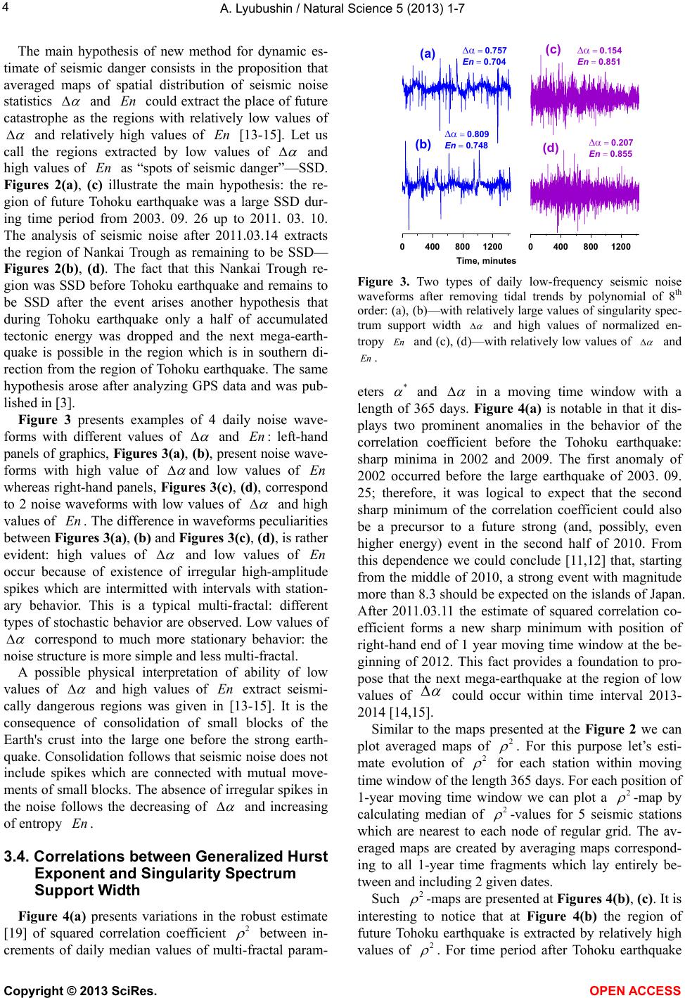

A. Lyubushin / Natural Science 5 (2013) 1-7

The main hypothesis of new method for dynamic es-

timate of seismic danger consists in the proposition that

averaged maps of spatial distribution of seismic noise

statistics



 and could extract the place of future

catastrophe as the regions with relatively low values of



 and relatively high values of [13-15]. Let us

call the regions extracted by low values of





and

high values of as “spots of seismic danger”—SSD.

Figures 2(a), (c) illustrate the main hypothesis: the re-

gion of future Tohoku earthquake was a large SSD dur-

ing time period from 2003. 09. 26 up to 2011. 03. 10.

The analysis of seismic noise after 2011.03.14 extracts

the region of Nankai Trough as remaining to be SSD—

Figures 2(b), (d). The fact that this Nankai Trough re-

gion was SSD before Tohoku earthquake and remains to

be SSD after the event arises another hypothesis that

during Tohoku earthquake only a half of accumulated

tectonic energy was dropped and the next mega-earth-

quake is possible in the region which is in southern di-

rection from the region of Tohoku earthquake. The same

hypothesis arose after analyzing GPS data and was pub-

lished in [3].

Figure 3 presents examples of 4 daily noise wave-

forms with different values of



 and : left-hand

panels of graphics, Figures 3(a), (b), present noise wave-

forms with high value of



and low values of

whereas right-hand panels, Figures 3(c), (d), correspond

to 2 noise waveforms with low values of



 and high

values of . The difference in waveforms peculiarities

between Figures 3(a), (b) and Figures 3(c), (d), is rath er

evident: high values of



 and low values of

occur because of existence of irregular high-amplitude

spikes which are intermitted with intervals with station-

ary behavior. This is a typical multi-fractal: different

types of stochastic behavior are observed. Low values of



 correspond to much more stationary behavior: the

noise structure is more simple and less multi-fractal.

A possible physical interpretation of ability of low

values of



 and high values of extract seismi-

cally dangerous regions was given in [13-15]. It is the

consequence of consolidation of small blocks of the

Earth's crust into the large one before the strong earth-

quake. Consolidation follows that seismic noise does not

include spikes which are connected with mutual move-

ments of small blocks. The absence of irregular spikes in

the noise follows the decreasing of



 and increasing

of entropy .

3.4. Correlations between Generalized Hurst

Exponent and Singularity Spectrum

Support Width

Figure 4(a) presents variations in the robust estimate

[19] of squared correlation coefficient 2



between in-

crements of daily median values of multi-fractal param-

0400800 12000400800 1200





0.757



0.704





0.809



0.748





0.207



0.855





0.154



0.851

ime,minutes

(a)

(b)

(c)

(d)

Figure 3. Two types of daily low-frequency seismic noise

waveforms after removing tidal trends by polynomial of 8th

order: (a), (b)—with relatively large values of singularity spec-

trum support width





and high values of normalized en-

tropy and (c), (d)—with relatively low values of En





and

eters *



and





in a moving time window with a

length of 365 days. Figure 4(a) is notable in that it dis-

plays two prominent anomalies in the behavior of the

correlation coefficient before the Tohoku earthquake:

sharp minima in 2002 and 2009. The first anomaly of

2002 occurred before the large earthquake of 2003. 09.

25; therefore, it was logical to expect that the second

sharp minimum of the correlation coefficient could also

be a precursor to a future strong (and, possibly, even

higher energy) event in the second half of 2010. From

this dependence we could conclude [11,12] that, starting

from the middle of 2010, a strong event with magnitude

more than 8.3 should be expected on the islands of Japan.

After 2011.03.11 the estimate of squared correlation co-

efficient forms a new sharp minimum with position of

right-hand end of 1 year moving time window at the be-

ginning of 2012. This fact provides a foundation to pro-

pose that the next mega-earthquake at the region of low

values of





could occur within time interval 2013-

2014 [14,15].

Similar to the maps presented at the Figure 2 we can

plot averaged maps of 2



. For this purpose let’s esti-

mate evolution of 2



for each station within moving

time window of the length 365 days. For each position of

1-year moving time window we can plot a 2



-map by

calculating median of 2



-values for 5 seismic stations

which are nearest to each node of regular grid. The av-

eraged maps are created by averaging maps correspond-

ing to all 1-year time fragments which lay entirely be-

tween and including 2 given dates.

Such 2



-maps are presented at Figures 4(b), (c). It is

interesting to notice that at Figure 4(b) the region of

future Tohoku earthquake is extracted by relatively high

values of 2



. For time period after Tohoku earthquake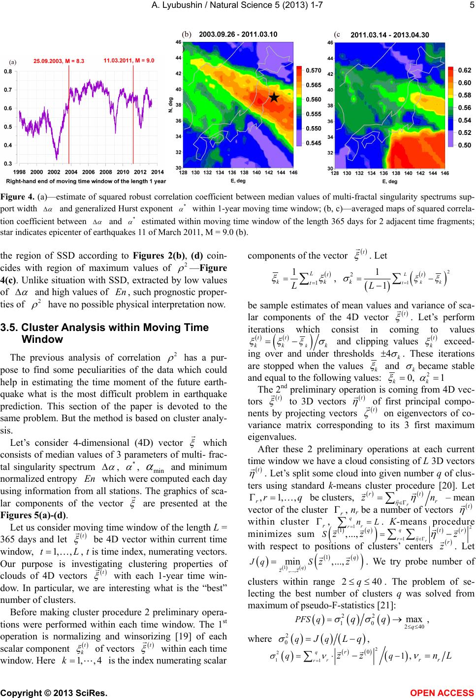

A. Lyubushin / Natural Science 5 (2013) 1-7 5

Figure 4. (a)—estimate of squared robust correlation coefficient between median values of multi-fractal singularity spectrums sup-

port width



 and generalized Hurst exponent *



within 1-year moving time window; (b, c)—averaged maps of squared correla-

tion coefficient between



 and *



estimated within moving time window of the length 365 days for 2 adjacent time fragments;

star indicates epicenter of earthquakes 11 of March 2011, M = 9.0 (b).

the region of SSD according to Figures 2(b), (d) coin-

cides with region of maximum values of 2



—Figure

4(c). Unlike situation with SSD, extracted by low values



 and high values of , such prognos tic proper-

ties of En



have no possible physical interpretation now.

3.5. Cluster Anal ysis within Moving Time

Window

The previous analysis of correlation 2



has a pur-

pose to find some peculiarities of the data which could

help in estimating the time moment of the future earth-

quake what is the most difficult problem in earthquake

prediction. This section of the paper is devoted to the

same problem. But the method is based on cluster analy-

sis.

Let’s consider 4-dimensional (4D) vector





which

consists of median values of 3 parameters of multi- frac-

tal singularity spectrum



, *



, min



and minimum

normalized entropy which were computed each day

using information from all stations. The graphics of sca-

lar components of the vector



 are presented at the

Figures 5(a)-(d).

Let us consider moving time window of the length L =

365 days and let







, be 4D vector within current time

window, , t is time index, numerating vectors.

Our purpose is investigating clustering properties of

clouds of 4D vectors

1,tL





 with each 1-year time win-

dow. In particular, we are interesting what is the “best”

number of clus te rs.

Before making cluster procedure 2 preliminary opera-

tions were performed within each time window. The 1st

operation is normalizing and winsorizing [19] of each

scalar component





of vectors





 within each time

window. Here is the index numerating scalar

1,, 4k

components of the vector







. Let



1Lt





,













be sample estimates of mean values ad variance of sca-

lar components of the 4D vector n





. Let’s perform

iterations which consist in coming to values

 





kk k





 and clipping values





exceed-

ing over and under thresholds 4k



. These iterations

are stopped when the values k



and k



became stable

and equal to the following values: 2



0,



The 2nd preliminary op eration is coming from 4D vec-

tors







to 3D vectors







of first principal compo-

nents by projecting vectors





 on eigenvectors of co-

variance matrix corresponding to its 3 first maximum

eigenvalues.

After these 2 preliminary operations at each current

time window we have a cloud consisting of L 3D vectors







. Let’s split some cloud into given number q of clus-

ters using standard k-means cluster procedure [20]. Let

,1,,r



 be clusters,

 



 – mean

vector of the cluster









, nr be a number of vectors







within cluster r



, . K-means procedure

minimizes sum 1

rnL



 









 





1,...,zzq

qtr











with respect to positions of clusters’ centers





. Let



 





1,...,

min ,...,

Jq Szz



. We try probe number of

clusters within range 2q40



. The problem of se-

lecting the best number of clusters q was solved from

maximum of pseudo-F-statistics [21]:









10 240

max

PFS qqq





,

where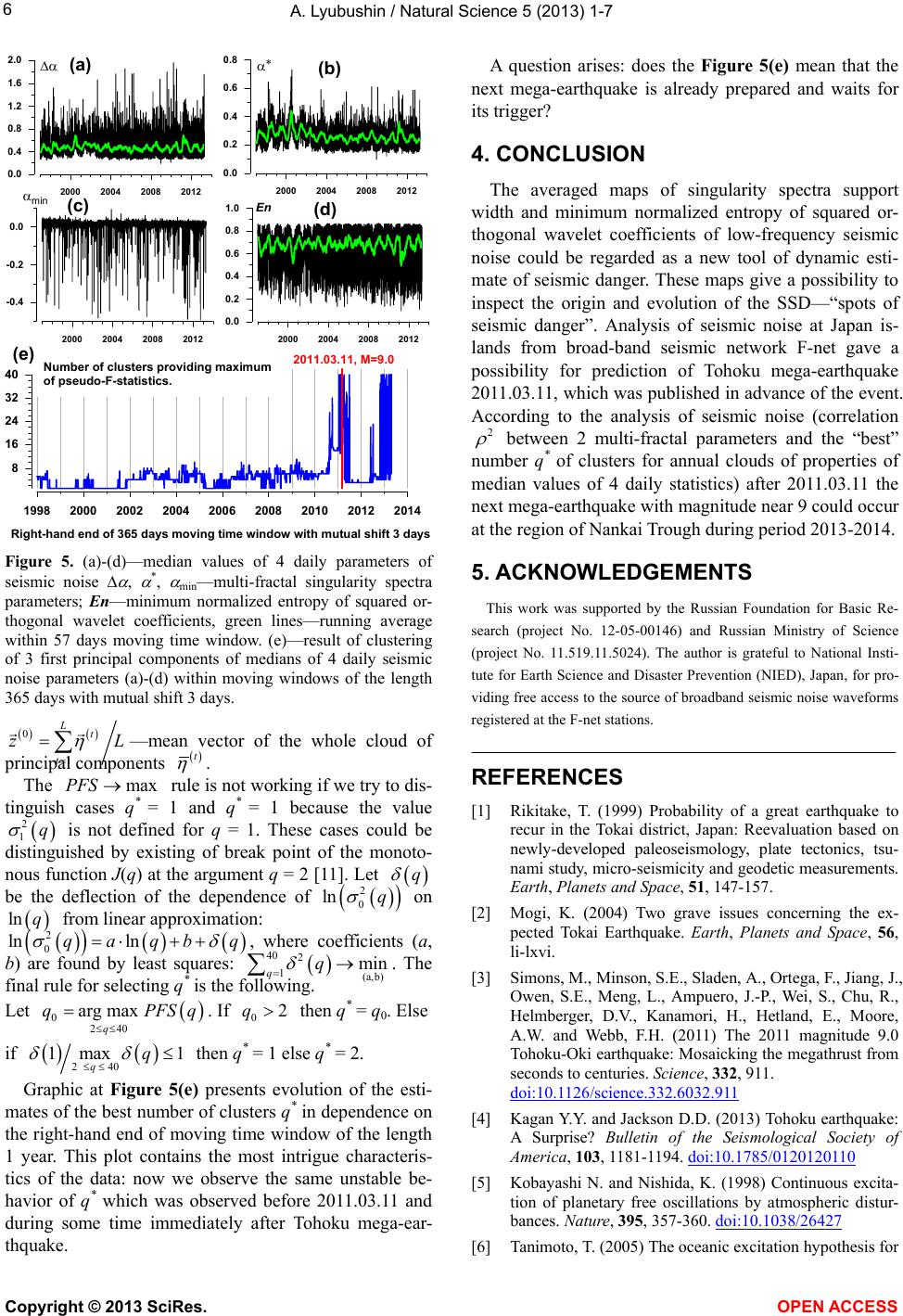













0qq





,



 



01,

qqzz n







 

L



A. Lyubushin / Natural Science 5 (2013) 1-7

2000 2004 2008 2012

0.0

0.4

0.8

1.2

1.6

2.0

2000 2004 2008 2012

0.0

0.2

0.4

0.6

0.8

2000200420082012

-0.4

-0.2

0.0

2000 2004 2008 2012

0.0

0.2

0.4

0.6

0.8

1.0

 





min

1998 2000 2002 2004 2006 2008 2010 2012 2014

40 2011.03.11, M=9.0

Right-hand end of 365 days moving time window with mutual shift 3 days

Number of clusters providing maximum

of pseudo-F-statistics.

(a) (b)

(e)

Figure 5. (a)-(d)—median values of 4 daily parameters of

seismic noise 



min—multi-fractal singularity spectra

parameters; En—minimum normalized entropy of squared or-

thogonal wavelet coefficients, green lines—running average

within 57 days moving time window. (e)—result of clustering

of 3 first principal components of medians of 4 daily seismic

noise parameters (a)-(d) within moving windows of the length

365 days with mutual shift 3 days.

 

1t

—mean vector of the whole cloud of

principal components











The rule is not working if we try to dis-

tinguish cases q* = 1 and q* = 1 because the value

is not defined for q = 1. These cases could be

distinguished by existing of break point of the monoto-

nous function J(q) at the argument q = 2 [11]. Let

maxPFS 











be the deflection of the dependence of











(a,b)

miq

from linear approximation:

, where coefficients (a,

b) are found by least squares: 1q. The

final rule for selecting q* is the following.



ln q



lnqa







qb q



S. If

40 2





Let then q* = q0. Else



0240

arg max

qPF



q

02q

 

240

1max 1



  then q* = 1 else q* = 2.

Graphic at Figure 5(e) presents evolution of the esti-

mates of the best number of clusters q* in dependence on

the right-hand end of moving time window of the length

1 year. This plot contains the most intrigue characteris-

tics of the data: now we observe the same unstable be-

havior of q* which was observed before 2011.03.11 and

during some time immediately after Tohoku mega-ear-

thquake.

A question arises: does the Figure 5(e) mean that the

next mega-earthquake is already prepared and waits for

its trigger?

4. CONCLUSION

The averaged maps of singularity spectra support

width and minimum normalized entropy of squared or-

thogonal wavelet coefficients of low-frequency seismic

noise could be regarded as a new tool of dynamic esti-

mate of seismic danger. These maps give a possibility to

inspect the origin and evolution of the SSD—“spots of

seismic danger”. Analysis of seismic noise at Japan is-

lands from broad-band seismic network F-net gave a

possibility for prediction of Tohoku mega-earthquake

2011.03.11, which was published in advance of the event.

According to the analysis of seismic noise (correlation



between 2 multi-fractal parameters and the “best”

number q* of clusters for annual clouds of properties of

median values of 4 daily statistics) after 2011.03.11 the

next mega-earthquake with magnitude near 9 could occur

at the region of Nankai Trough during peri od 20 1 3-2 01 4.

5. ACKNOWLEDGEMENTS

This work was supported by the Russian Foundation for Basic Re-

search (project No. 12-05-00146) and Russian Ministry of Science

(project No. 11.519.11.5024). The author is grateful to National Insti-

tute for Earth Science and Disaster Prevention (NIED), Japan, for pro-

viding free access to the source of broadband seismic noise waveforms

registered at the F-net stations.

REFERENCES

[1] Rikitake, T. (1999) Probability of a great earthquake to

recur in the Tokai district, Japan: Reevaluation based on

newly-developed paleoseismology, plate tectonics, tsu-

nami study, micro-seismicity and geodetic measurements.

Earth, Planets and Space, 51, 147-157.

[2] Mogi, K. (2004) Two grave issues concerning the ex-

pected Tokai Earthquake. Earth, Planets and Space, 56,

li-lxvi.

[3] Simons, M., Minson, S.E., Sladen, A., Ortega, F., Jiang, J.,

Owen, S.E., Meng, L., Ampuero, J.-P., Wei, S., Chu, R.,

Helmberger, D.V., Kanamori, H., Hetland, E., Moore,

A.W. and Webb, F.H. (2011) The 2011 magnitude 9.0

Tohoku-Oki earthquake: Mosaicking the megathrust from

seconds to centuries. Scienc e, 332, 911.

doi:10.1126/science.332.6032.911

[4] Kagan Y.Y. and Jackson D.D. (2013) Tohoku earthquake:

A Surprise? Bulletin of the Seismological Society of

America, 103, 1181-1194. doi:10.1785/0120120110

[5] Kobayashi N. and Nishida, K. (1998) Continuous excita-

tion of planetary free oscillations by atmospheric distur-

bances. Nature, 395, 357-360. doi:10.1038/26427

[6] Tanimoto, T. (2005) The oceanic excitation hypothesis for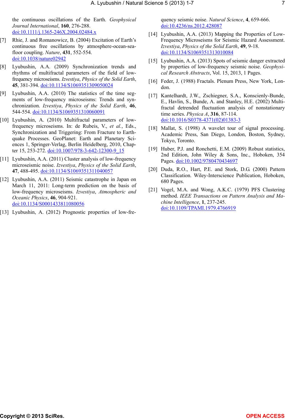

A. Lyubushin / Natural Science 5 (2013) 1-7

the continuous oscillations of the Earth. Geophysical

Journal International, 160, 276-288.

d oi:10.1111/j.1365-246X.2004.02484.x

[7] Rhie, J. and Romanowicz, B. (2004) Excitation of Earth’s

continuous free oscillations by atmosphere-ocean-sea-

floor coupling. Nature, 431, 552-554.

doi:10.1038/nature02942

[8] Lyubushin, A.A. (2009) Synchronization trends and

rhythms of multifractal parameters of the field of low-

frequency microseisms. Izvestiya, Physics of the Solid Earth,

45, 381-394. doi:10.1134/S1069351309050024

[9] Lyubushin, A.A. (2010) The statistics of the time seg-

ments of low-frequency microseisms: Trends and syn-

chronization. Izvestiya, Physics of the Solid Earth, 46,

544-554. doi:10.1134/S1069351310060091

[10] Lyubushin, A. (2010) Multifractal parameters of low-

frequency microseisms. In: de Rubeis, V., et al., Eds.,

Synchronization and Triggering: From Fracture to Earth-

quake Processes. GeoPlanet: Earth and Planetary Sci-

ences 1, Springer-Verlag, Berlin Heidelberg, 2010, Chap-

ter 15, 253-272. doi:10.1007/978-3-642-12300-9_15

[11] Lyubushin, A.A. (2011) Cluster analysis of low-frequency

microseismic noise. Izvestiya, Physics of the Solid Earth,

47, 488-495. doi:10.1134/S1069351311040057

[12] Lyubushin, A.A. (2011) Seismic catastrophe in Japan on

March 11, 2011: Long-term prediction on the basis of

low-frequency microseisms. Izvestiya, Atmospheric and

Oceanic Physics, 46, 904-921.

doi:10.1134/S0001433811080056

[13] Lyubushin, A. (2012) Prognostic properties of low-fre-

quency seismic noise. Natural Science, 4, 659-666.

doi:10.4236/ns.2012.428087

[14] Lyubushin, A.A. (2013) Mapping the Properties of Low-

Frequency Microseisms for Seismic Hazard Assessment.

Izvestiya, Physics of the Solid Earth, 49, 9-18.

doi:10.1134/S1069351313010084

[15] Lyubushin, A.A. (2013) Spots of seismic danger extracted

by properties of low-frequency seismic noise. Geophysi-

cal Research Abstracts, Vol. 15, 2013, 1 Pages.

[16] Feder, J. (1988) Fractals. Plenum Press, New York, Lon-

don.

[17] Kantelhardt, J.W., Zschiegner, S.A., Konscienly-Bunde,

E., Havlin, S., Bunde, A. and Stanley, H.E. (2002) Multi-

fractal detrended fluctuation analysis of nonstationary

time series. Physica A, 316, 87-114.

doi:10.1016/S0378-4371(02)01383-3

[18] Mallat, S. (1998) A wavelet tour of signal processing.

Academic Press, San Diego, London, Boston, Sydney,

Tokyo, Toronto.

[19] Huber, P.J. and Ronchetti, E.M. (2009) Robust statistics,

2nd Edition, John Wiley & Sons, Inc., Hoboken, 354

Pages. doi:10.1002/9780470434697

[20] Duda, R.O., Hart, P.E. and Stork, D.G. (2000) Pattern

Classification. Wiley-Interscience Publication, Hoboken,

680 Pages.

[21] Vogel, M.A. and Wong, A.K.C. (1979) PFS Clustering

method. IEEE Transactions on Pattern Analysis and Ma-

chine Intelligence, 1, 237-245.

doi:10.1109/TPAMI.1979.4766919