Impact of Forecast Errors in CPFR Collaboration Strategy

doi:10.4236/ajibm.2013.34046

Paper Menu >>

Journal Menu >>

American Journal of Industrial and Business Management, 2013, 3, 389-394

http://dx.doi.org/10.4236/ajibm.2013.34046 Published Online August 2013 (http://www.scirp.org/journal/ajibm)

389

Impact of Forecast Errors in CPFR Collaboration Strategy

Kamalapur Raj

University of Wisconsin Oshkosh, Wisconsin, USA.

Email: [email protected]

Received May 24th, 2013; revised June 24th, 2013; accepted July 16th, 2013

permits unrestricted use, distribution, and reproduction in any medium, provided the original work is properly cited.

ABSTRACT

The primary objective of this research is to investigate the impact of random forecast error and bias forecast error in

Collaborative Planning, Forecasting and Replenishment (CPFR) strategy on the cost of inventory management for both

the manufacturer and retailer. Discrete-event simulation is used to develop a CPFR collaboration model where forecast,

sales and inventory level information is shared between a retailer and a manufacturer. Based on the results of this study,

we conclude that the higher random forecast error and negative bias forecast error increases the cost of inventory man-

agement for both the manufacturer and the retailer. When demand variability is high, a bias forecast error has a bigger

impact on inventory management cost compared to a random forecast error for both the manufacturer and retailer. Also,

a positive bias forecast error is more beneficial than a negative bias forecast error to gain maximum benefits of CPFR

strategy.

Keywords: CPFR Collaboration Strategy; Inventory Management; Simulation Modeling

1. Introduction

Inventory is a significant and often one of the largest

assets for most companies. To provide good customer

service, many supply chain members maintain a high

level of safety stock inventory which increases the total

cost in the supply chain. For example, in 1996, approxi-

mately $700 billion of the $2.3 trillion retail supply chain

was in safety stock inventory [1]. Also, in recent Annual

State of Logistics Report, over $1 trillion was annually

spent on logistics, with approximately 33 percent being

attributed to the cost of holding inventory [2]. So in re-

cent years, academic researchers and practitioners have

emphasized that information sharing between supply

chain members can significantly reduce inventory levels

and improve service levels in the supply chain. In order

to encourage retailers to share information with manufac-

turers, collaboration strategies like Vendor Managed In-

ventory (VMI) and Collaborative Planning, Forecasting

and Replenishment (CPFR) have been developed and

implemented in many industries with mixed results [3,4].

Since a supply chain is a complex network, many re-

searchers consider the dyadic structure (two-levels) to

study the benefits of information sharing. Many research

studies have shown the benefits of demand information

sharing in the supply chain [5-7]. Most of these studies

assume that the retailer knows the exact customer de-

mand in the supply chain. However in a variable demand

environment, the retailer may not know the exact cus-

tomer demand and have to develop their demand forecast.

Retailers generally use different forecasting methods and

this can impact the forecast accuracy of the customer

demand. So the benefit of information sharing greatly

depends on the forecast accuracy of the customer de-

mand in a variable demand environment. There are some

studies that consider the impact of forecast errors on the

value of information sharing. One research study [8] uses

simulation modeling to investigate the impact of fore-

casting errors on the value of information sharing in a

supply chain with four retailers and a manufacturer. They

show that forecast errors have an impact on the value of

information sharing. Their study only considered forecast

information sharing between the supply chain partners.

However in a CPFR strategy, along with forecast data,

generally sales data and inventory level information is

shared between the supply chain partners. There are no

studies that consider the impact of forecast errors on the

cost of inventory management in CPFR collaboration

strategy for both the manufacturer and retailer in a vari-

able demand environment. This study uses discrete-event

simulation to develop a CPFR collaboration model where

forecast, sales and inventory level information is shared

between a retailer and a manufacturer. Using this simula-

tion model, we investigate the impact of random forecast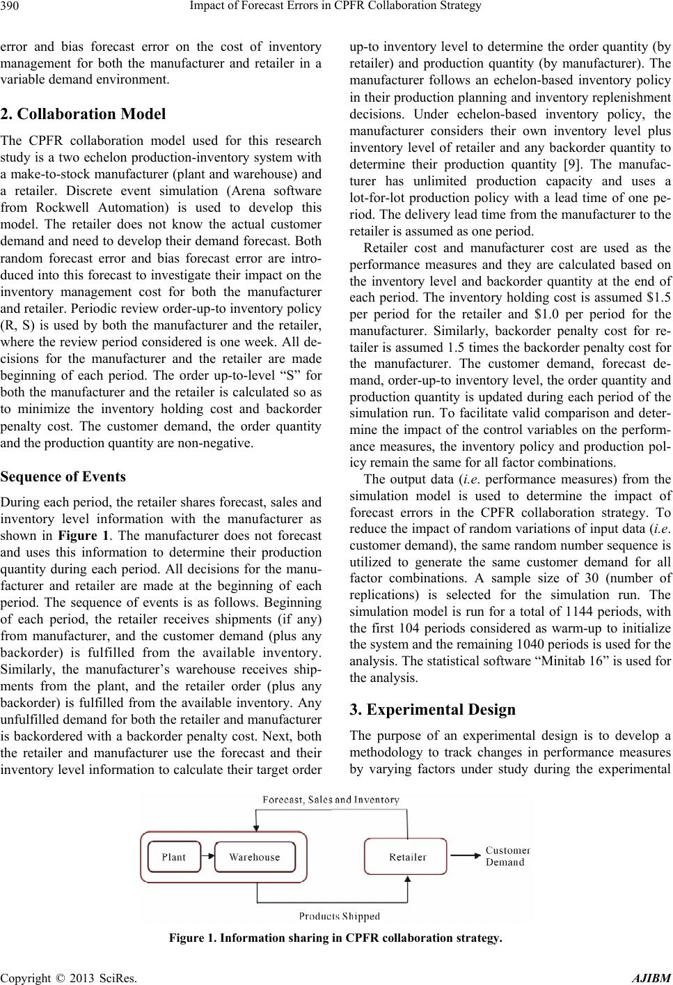

Impact of Forecast Errors in CPFR Collaboration Strategy

390

error and bias forecast error on the cost of inventory

management for both the manufacturer and retailer in a

variable demand environment.

2. Collaboration Model

The CPFR collaboration model used for this research

study is a two echelon production-inventory system with

a make-to-stock manufacturer (plant and warehouse) and

a retailer. Discrete event simulation (Arena software

from Rockwell Automation) is used to develop this

model. The retailer does not know the actual customer

demand and need to develop their demand forecast. Both

random forecast error and bias forecast error are intro-

duced into this forecast to investigate their impact on the

inventory management cost for both the manufacturer

and retailer. Periodic review order-up-to inventory policy

(R, S) is used by both the manufacturer and the retailer,

where the review period considered is one week. All de-

cisions for the manufacturer and the retailer are made

beginning of each period. The order up-to-level “S” for

both the manufacturer and the retailer is calculated so as

to minimize the inventory holding cost and backorder

penalty cost. The customer demand, the order quantity

and the production quantity are non-negative.

Sequence of Events

During each period, the retailer shares forecast, sales and

inventory level information with the manufacturer as

shown in Figure 1. The manufacturer does not forecast

and uses this information to determine their production

quantity during each period. All decisions for the manu-

facturer and retailer are made at the beginning of each

period. The sequence of events is as follows. Beginning

of each period, the retailer receives shipments (if any)

from manufacturer, and the customer demand (plus any

backorder) is fulfilled from the available inventory.

Similarly, the manufacturer’s warehouse receives ship-

ments from the plant, and the retailer order (plus any

backorder) is fulfilled from the available inventory. Any

unfulfilled demand for both the retailer and manufacturer

is backordered with a backorder penalty cost. Next, both

the retailer and manufacturer use the forecast and their

inventory level information to calculate their target order

up-to inventory level to determine the order quantity (by

retailer) and production quantity (by manufacturer). The

manufacturer follows an echelon-based inventory policy

in their production planning and inventory replenishment

decisions. Under echelon-based inventory policy, the

manufacturer considers their own inventory level plus

inventory level of retailer and any backorder quantity to

determine their production quantity [9]. The manufac-

turer has unlimited production capacity and uses a

lot-for-lot production policy with a lead time of one pe-

riod. The delivery lead time from the manufacturer to the

retailer is assumed as one period.

Retailer cost and manufacturer cost are used as the

performance measures and they are calculated based on

the inventory level and backorder quantity at the end of

each period. The inventory holding cost is assumed $1.5

per period for the retailer and $1.0 per period for the

manufacturer. Similarly, backorder penalty cost for re-

tailer is assumed 1.5 times the backorder penalty cost for

the manufacturer. The customer demand, forecast de-

mand, order-up-to inventory level, the order quantity and

production quantity is updated during each period of the

simulation run. To facilitate valid comparison and deter-

mine the impact of the control variables on the perform-

ance measures, the inventory policy and production pol-

icy remain the same for all factor combinations.

The output data (i.e. performance measures) from the

simulation model is used to determine the impact of

forecast errors in the CPFR collaboration strategy. To

reduce the impact of random variations of input data (i.e.

customer demand), the same random number sequence is

utilized to generate the same customer demand for all

factor combinations. A sample size of 30 (number of

replications) is selected for the simulation run. The

simulation model is run for a total of 1144 periods, with

the first 104 periods considered as warm-up to initialize

the system and the remaining 1040 periods is used for the

analysis. The statistical software “Minitab 16” is used for

the analysis.

3. Experimental Design

The purpose of an experimental design is to develop a

methodology to track changes in performance measures

by varying factors under study during the experimental

Figure 1. Information sharing in CPFR collaboration strategy.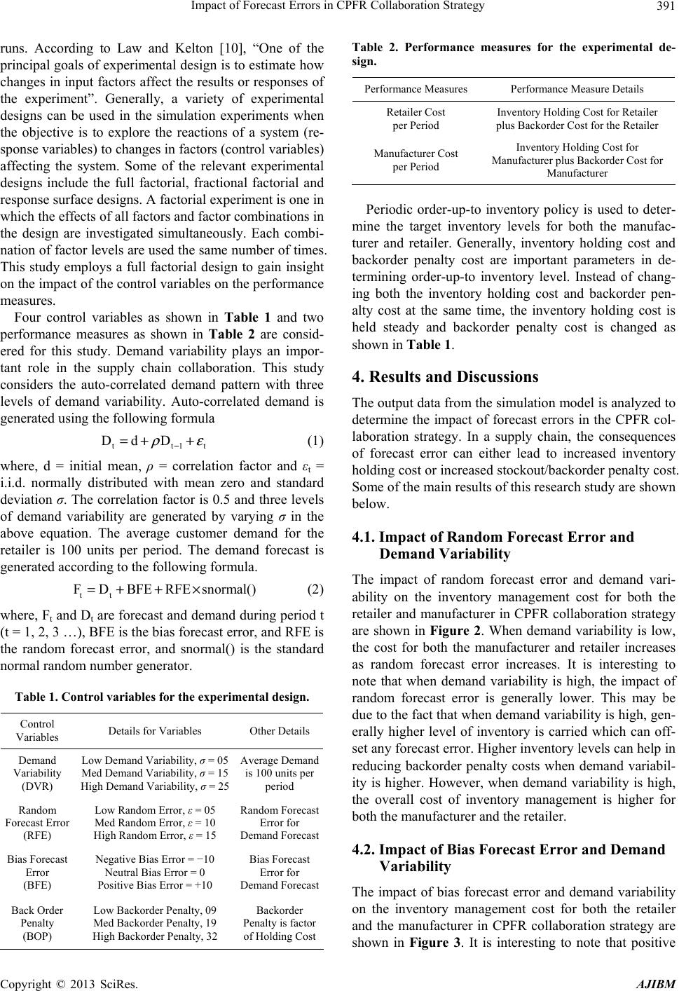

Impact of Forecast Errors in CPFR Collaboration Strategy 391

runs. According to Law and Kelton [10], “One of the

principal goals of experimental design is to estimate how

changes in input factors affect the results or responses of

the experiment”. Generally, a variety of experimental

designs can be used in the simulation experiments when

the objective is to explore the reactions of a system (re-

sponse variables) to changes in factors (control variables)

affecting the system. Some of the relevant experimental

designs include the full factorial, fractional factorial and

response surface designs. A factorial experiment is one in

which the effects of all factors and factor combinations in

the design are investigated simultaneously. Each combi-

nation of factor levels are used the same number of times.

This study employs a full factorial design to gain insight

on the impact of the control variables on the performance

measures.

Four control variables as shown in Table 1 and two

performance measures as shown in Table 2 are consid-

ered for this study. Demand variability plays an impor-

tant role in the supply chain collaboration. This study

considers the auto-correlated demand pattern with three

levels of demand variability. Auto-correlated demand is

generated using the following formula

tt1

Dd Dt

−

=++ (1)

where, d = initial mean, ρ = correlation factor and εt =

i.i.d. normally distributed with mean zero and standard

deviation σ. The correlation factor is 0.5 and three levels

of demand variability are generated by varying σ in the

above equation. The average customer demand for the

retailer is 100 units per period. The demand forecast is

generated according to the following formula.

FDBFERFEsnorml(a)=++ × (2)

where, Ft and Dt are forecast and demand during period t

(t = 1, 2, 3 …), BFE is the bias forecast error, and RFE is

the random forecast error, and snormal() is the standard

normal random number generator.

Table 1. Control variables for the experimental design.

Control

Variables Details for Variables Other Details

Demand

Variability

(DVR)

Low Demand Variability, σ = 05

Med Demand Variability, σ = 15

High Demand Variability, σ = 25

Average Demand

is 100 units per

period

Random

Forecast Error

(RFE)

Low Random Error, ε = 05

Med Random Error, ε = 10

High Random Error, ε = 15

Random Forecast

Error for

Demand Forecast

Bias Forecast

Error

(BFE)

Negative Bias Error = −10

Neutral Bias Error = 0

Positive Bias Error = +10

Bias Forecast

Error for

Demand Forecast

Back Order

Penalty

(BOP)

Low Backorder Penalty, 09

Med Backorder Penalty, 19

High Backorder Penalty, 32

Backorder

Penalty is factor

of Holding Cost

Table 2. Performance measures for the experimental de-

sign.

Performance Measures Performance Measure Details

Retailer Cost

per Period

Inventory Holding Cost for Retailer

plus Backorder Cost for the Retailer

Manufacturer Cost

per Period

Inventory Holding Cost for

Manufacturer plus Backorder Cost for

Manufacturer

Periodic order-up-to inventory policy is used to deter-

mine the target inventory levels for both the manufac-

turer and retailer. Generally, inventory holding cost and

backorder penalty cost are important parameters in de-

termining order-up-to inventory level. Instead of chang-

ing both the inventory holding cost and backorder pen-

alty cost at the same time, the inventory holding cost is

held steady and backorder penalty cost is changed as

shown in Table 1.

4. Results and Discussions

The output data from the simulation model is analyzed to

determine the impact of forecast errors in the CPFR col-

laboration strategy. In a supply chain, the consequences

of forecast error can either lead to increased inventory

holding cost or increased stockout/backorder penalty cost.

Some of the main results of this research study are shown

below.

4.1. Impact of Random Forecast Error and

Demand Variability

The impact of random forecast error and demand vari-

ability on the inventory management cost for both the

retailer and manufacturer in CPFR collaboration strategy

are shown in Figure 2. When demand variability is low,

the cost for both the manufacturer and retailer increases

as random forecast error increases. It is interesting to

note that when demand variability is high, the impact of

random forecast error is generally lower. This may be

due to the fact that when demand variability is high, gen-

erally higher level of inventory is carried which can off-

set any forecast error. Higher inventory levels can help in

reducing backorder penalty costs when demand variabil-

ity is higher. However, when demand variability is high,

the overall cost of inventory management is higher for

both the manufacturer and the retailer.

4.2. Impact of Bias Forecast Error and Demand

Variability

The impact of bias forecast error and demand variability

on the inventory management cost for both the retailer

and the manufacturer in CPFR collaboration strategy are

shown in Figure 3. It is interesting to note that positive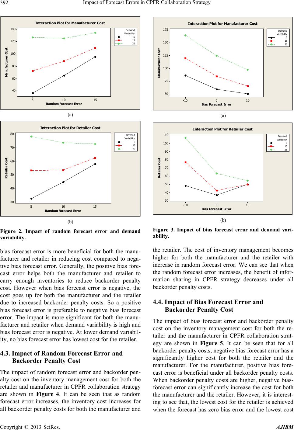

Impact of Forecast Errors in CPFR Collaboration Strategy

392

15105

140

120

100

Random Forecast Error

Manufacturer Cost

Variability

Demand

Interaction Plot for Manufacturer Cost

(a)

15105

Random Forecast Error

Retailer Cost

Var ia b ility

Demand

Interaction Plot for Retailer Cost

(b)

Figure 2. Impact of random forecast error and demand

variability.

bias forecast error is more beneficial for both the manu-

facturer and retailer in reducing cost compared to nega-

tive bias forecast error. Generally, the positive bias fore-

cast error helps both the manufacturer and retailer to

carry enough inventories to reduce backorder penalty

cost. However when bias forecast error is negative, the

cost goes up for both the manufacturer and the retailer

due to increased backorder penalty costs. So a positive

bias forecast error is preferable to negative bias forecast

error. The impact is more significant for both the manu-

facturer and retailer when demand variability is high and

bias forecast error is negative. At lower demand variabil-

ity, no bias forecast error has lowest cost for the retailer.

4.3. Impact of Random Forecast Error and

Backorder Penalty Cost

The impact of random forecast error and backorder pen-

alty cost on the inventory management cost for both the

retailer and manufacturer in CPFR collaboration strategy

are shown in Figure 4. It can be seen that as random

forecast error increases, the inventory cost increases for

all backorder penalty costs for both the manufacturer and

100-10

175

150

125

100

Bias Forecast Error

Manufacturer Cost

Variability

Demand

Interaction Plot for Manufacturer Cost

(a)

100-10

110

100

Bias Forecast Error

Retailer Cost

Variability

Demand

Interaction Plot for Retailer Cost

(b)

Figure 3. Impact of bias forecast error and demand vari-

ability.

the retailer. The cost of inventory management becomes

higher for both the manufacturer and the retailer with

increase in random forecast error. We can see that when

the random forecast error increases, the benefit of infor-

mation sharing in CPFR strategy decreases under all

backorder penalty costs.

4.4. Impact of Bias Forecast Error and

Backorder Penalty Cost

The impact of bias forecast error and backorder penalty

cost on the inventory management cost for both the re-

tailer and the manufacturer in CPFR collaboration strat-

egy are shown in Figure 5. It can be seen that for all

backorder penalty costs, negative bias forecast error has a

significantly higher cost for both the retailer and the

manufacturer. For the manufacturer, positive bias fore-

cast error is beneficial under all backorder penalty costs.

When backorder penalty costs are higher, negative bias-

forecast error can significantly increase the cost for both

the manufacturer and the retailer. However, it is interest-

ing to see that, the lowest cost for the retailer is achieved

when the forecast has zero bias error and the lowest cost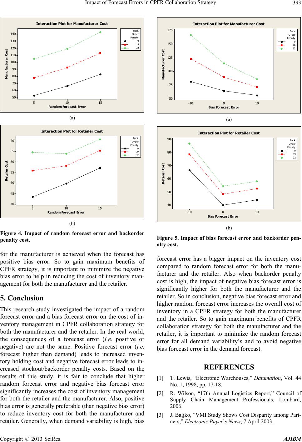

Impact of Forecast Errors in CPFR Collaboration Strategy 393

15105

140

130

120

110

100

Random Forecast Error

Manufacturer Cost

Penalty

Order

Back

Interaction Plot for Manufacturer Cost

(a)

15105

Random Forecast Error

Retailer Cost

Penalty

Order

Back

Interaction Plot for Retailer Cost

(b)

Figure 4. Impact of random forecast error and backorder

penalty cost.

for the manufacturer is achieved when the forecast has

positive bias error. So to gain maximum benefits of

CPFR strategy, it is important to minimize the negative

bias error to help in reducing the cost of inventory man-

agement for both the manufacturer and the retailer.

5. Conclusion

This research study investigated the impact of a random

forecast error and a bias forecast error on the cost of in-

ventory management in CPFR collaboration strategy for

both the manufacturer and the retailer. In the real world,

the consequences of a forecast error (i.e. positive or

negative) are not the same. Positive forecast error (i.e.

forecast higher than demand) leads to increased inven-

tory holding cost and negative forecast error leads to in-

creased stockout/backorder penalty costs. Based on the

results of this study, it is fair to conclude that higher

random forecast error and negative bias forecast error

significantly increases the cost of inventory management

for both the retailer and the manufacturer. Also, positive

bias error is generally preferable (than negative bias error)

to reduce inventory cost for both the manufacturer and

retailer. Generally, when demand variability is high, bias

100-10

175

150

125

100

Bias Forecast Error

Manufacturer Cost

Penalty

Order

Back

Interaction Plot for Manufacturer Cost

(a)

100-10

Bias Forecast Error

Retailer Cost

Penalty

Order

Back

Interaction Plot for Retailer Cost

(b)

Figure 5. Impact of bias forecast error and backorder pen-

alty cost.

forecast error has a bigger impact on the inventory cost

compared to random forecast error for both the manu-

facturer and the retailer. Also when backorder penalty

cost is high, the impact of negative bias forecast error is

significantly higher for both the manufacturer and the

retailer. So in conclusion, negative bias forecast error and

higher random forecast error increases the overall cost of

inventory in a CPFR strategy for both the manufacturer

and the retailer. So to gain maximum benefits of CPFR

collaboration strategy for both the manufacturer and the

retailer, it is important to minimize the random forecast

error for all demand variability’s and to avoid negative

bias forecast error in the demand forecast.

REFERENCES

[1] T. Lewis, “Electronic Warehouses,” Datamation, Vol. 44

No. 1, 1998, pp. 17-18.

[2] R. Wilson, “17th Annual Logistics Report,” Council of

Supply Chain Management Professionals, Lombard,

2006.

[3] J. Baljko, “VMI Study Shows Cost Disparity among Part-

ners,” Electronic Buyer’s News, 7 April 2003.

Impact of Forecast Errors in CPFR Collaboration Strategy

394

[4] J. Cooke, “VMI: Very Mixed Impact,” Logistics Man-

agement and Distribution Report, Vol. 37, No. 12, 1998,

pp. 51-53.

[5] G. Cachon and M. Fisher, “Supply Chain Inventory Man-

agement and the Value of Shared Information,” Man-

agement Science, Vol. 46, No. 8, 2000, pp. 1032-1048.

doi:10.1287/mnsc.46.8.1032.12029

[6] H. Lee, K. So and C. Tang, “The Value of Information

Sharing in a Two Level Supply Chain,” Management Sci-

ence, Vol. 46, No. 5, 2000, pp. 626-643.

doi:10.1287/mnsc.46.5.626.12047

[7] Z. Yu, H. Yan and T. Cheng, “Benefits of Information

Sharing with Supply Chain Partnerships,” Industrial

Management & Data Systems, Vol. 101, No. 3, 2001, pp.

114-119. doi:10.1108/02635570110386625

[8] X. D. Zhao, et al., “The Impact of Forecast Errors on

Early Order Commitment in the Supply Chain,” Decision

Sciences, Vol. 33, No. 2, 2002, pp. 251-280.

doi:10.1111/j.1540-5915.2002.tb01644.x

[9] S. Axsater and K. Rosling, “Installation vs. Echelon

Stock Policies for Multilevel Inventory Control,” Man-

agement Science, Vol. 39, No 10, 1993, pp. 1274-1280.

doi:10.1287/mnsc.39.10.1274

[10] A. Law and W. Kelton, “Simulation Modeling and Analy-

sis,” 3rd Edition, McGraw Hill, New York, 2000.