Comparison of Iterative Wavefront Estimation Methods

doi:10.4236/opj.2013.32B022

Paper Menu >>

Journal Menu >>

Optics and Photonics Journal, 2013, 3, 86-89

doi:10.4236/opj.2013.32B022 Published Online June 2013 (http://www.scirp.org/journal/opj)

Comparison of Iterative Wavefront Estimation Methods*

Y. Pankratova, A. Larichev, N. Iroshnikov

Faculty of Physics, Lomonosov MSU, Moscow, Russian Federation

Email: [email protected], [email protected]

Received 2013

ABSTRACT

The iterative reconstruction methods of the wavefront phase estimation from a set of discrete phase slope measurements

have been considered. The values of the root-mean-square difference between the reconstructed and original wavefront

have been received for Jacobi, Gauss-Seidel, Successive over-relaxation and Successive over-relaxation with Simpson

Reconstructor methods. The method with the highest accuracy has been defined.

Keywords: Wavefront Estimation; Phase; Reconstruction; Iterative Methods

1. Introduction

Now methods of adaptive optics become more and more

widespread in optics. That appears to be particularly im-

portant for ultra-high intensity lasers as the number of

optical elements that this lasers include is rather high so

the appearance of static and thermo-induced aberrations

of the wavefront are possible [1], for diagnostic medical

systems for correction of the crystalline lens and corneal

aberrations[2] and for ground-based telescopes to correct

for the atmospheric aberrations. In this paper we consider

the comparison research of the iterative methods of esti-

mating wavefront phase from a set of discrete phase

slope measurements that was obtained from a Hartmann

sensor.

2. Shack-Hartmann Wavefront Sensor

2.1. Operation Principle

The Shack-Hartmann wavefront sensor contains a lenslet

array that consists of a two-dimensional array of a few

hundred lenslets all with the same diameter and the same

focal length. The light ray spatially sampled into many

individual beams by the lenslet array and forms multiple

spots in the focal plane of the lenslets. A CCD camera

placed in the focal plane of the lanslet array records the

spot array pattern for wavefront calculation. For a wave

with plane wavefront the Shack-Hartmann spots are

formed along the optical axis of each lenslet, resulting in

a regularly spaced grid of spots in the focal plane of the

lenslet array. In contrast, individual spots formed by

wavefront with aberrations are displaced from the optical

axis of each lenslet. The displacement of each spot is

proportional to the wavefront slope.[2]

2.2. Specific Features

Modern Shack-Hartmann sensors consist of a large

number of lenslets, this number can exceed 10000. While

using such sensors it's possible to face the problem of

crosstalk, limited aperture and the loss of some points.

Not all methods of wavefront estimation are suitable un-

der these conditions.

3. Wavefront Reconstruction Methods

As an example of reconstruction methods can be taken

modal and zonal wavefront reconstruction methods.

• In the modal approach the wavefront is expanded

into a set of orthogonal basis functions, and the coeffi-

cients of the set of basis functions are estimated from the

discrete phase-slope measurements. The appearance of

the large reconstruction error is possible.

• In the zonal approach, the wavefront is estimated

directly from a set of discrete phase-slope measurements.

Estimated with this method wavefront has less recon-

struction error then that in modal approach. For the zonal

reconstruction method the iterative algorithms may be

used.

4. Iterative Methods

4.1. Jacobi and Gauss-Seidel Methods

One of the first iterative methods are Jacobi and Gauss-

Seidel methods. These methods were proposed by South-

well for wavefront reconstruction. The idea behind this

method is to take into account the wavefront deformation

for some vertical and horizontal adjacent spots in the

calculation of the wavefront deformation for all spots.

Southwell proposed an iterative solution where for any

point (n,m) the wavefront is calculated with (1), (2) and

*Russian Foundation for Basic Research №11-02-01353-a.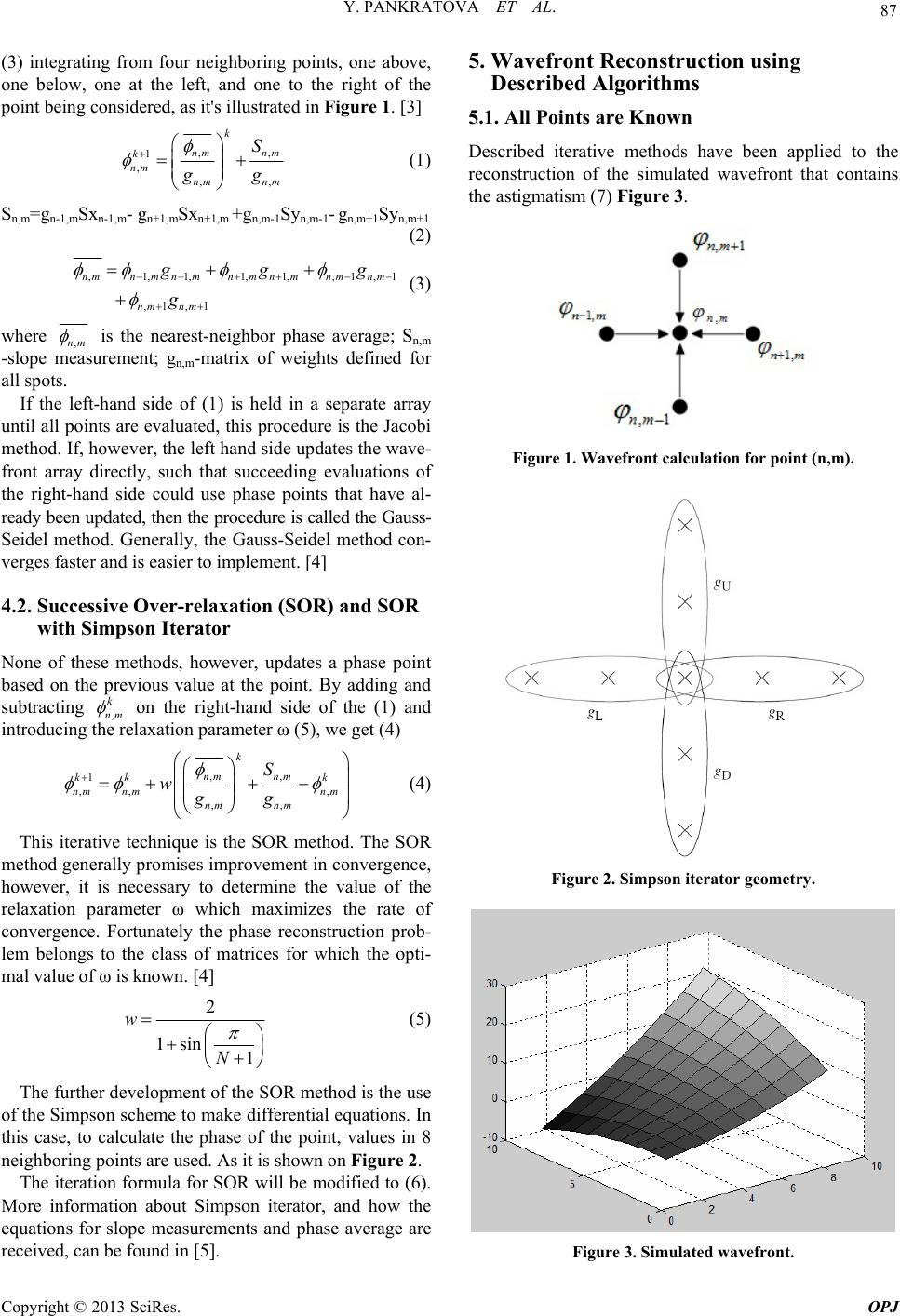

Y. PANKRATOVA ET AL. 87

(3) integrating from four neighboring points, one above,

one below, one at the left, and one to the right of the

point being considered, as it's illustrated in Figure 1. [3]

nm nm

nm nm nm











(1)

Sn,m=gn-1,mSxn-1,m- gn+1,mSxn+1,m +gn,m-1Syn,m-1- gn,m+1Syn,m+1

(2)

,1,1,1,1,,1,

,1 ,1

nmnmnmnmnmnm nm

nm nm

  



 









(3)

where ,nm



is the nearest-neighbor phase average; Sn,m

-slope measurement; gn,m-matrix of weights defined for

all spots.

If the left-hand side of (1) is held in a separate array

until all points are evaluated, this procedure is the Jacobi

method. If, however, the left hand side updates the wave-

front array directly, such that succeeding evaluations of

the right-hand side could use phase points that have al-

ready been updated, then the procedure is called the Gauss-

Seidel method. Generally, the Gauss-Seidel method con-

verges faster and is easier to implement. [4]

4.2. Successive Over-relaxation (SOR) and SOR

with Simpson Iterator

None of these methods, however, updates a phase point

based on the previous value at the point. By adding and

subtracting ,



on the right-hand side of the (1) and

introducing the relaxation parameter ω (5), we get (4)

,, ,

nm nm

kk k

nm nmnm

nm nm

wgg



 







 





(4)

This iterative technique is the SOR method. The SOR

method generally promises improvement in convergence,

however, it is necessary to determine the value of the

relaxation parameter ω which maximizes the rate of

convergence. Fortunately the phase reconstruction prob-

lem belongs to the class of matrices for which the opti-

mal value of ω is known. [4]

1sin 1











(5)

The further development of the SOR method is the use

of the Simpson scheme to make differential equations. In

this case, to calculate the phase of the point, values in 8

neighboring points are used. As it is shown on Figure 2.

The iteration formula for SOR will be modified to (6).

More information about Simpson iterator, and how the

equations for slope measurements and phase average are

received, can be found in [5].

5. Wavefront Reconstruction using

Described Algorithms

5.1. All Points are Known

Described iterative methods have been applied to the

reconstruction of the simulated wavefront that contains

the astigmatism (7) Figure 3.

Figure 1. Wavefront calculation for point (n,m).

Figure 2. Simpson iterator geometry.

Figure 3. Simulated wavefront.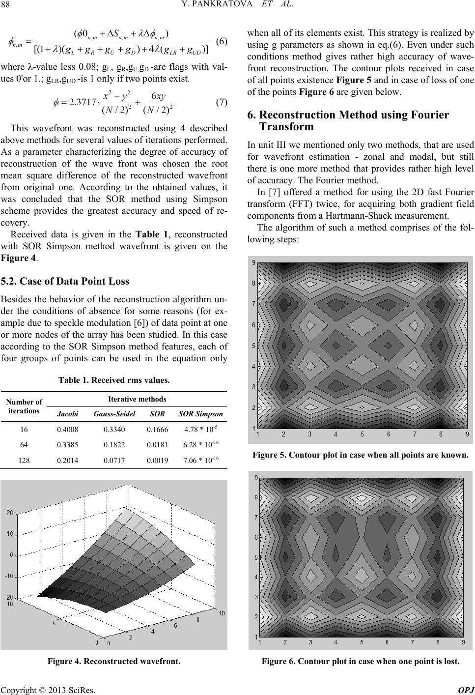

Y. PANKRATOVA ET AL.

,, ,

(0 )

[(1)()4 ()]

nm nmnm

nm LRUDLRUD

ggggg g





 

  (6)

where λ-value less 0.08; gL, gR,gU,gD -are flags with val-

ues 0'or 1.; gLR,gUD -is 1 only if two points exist.

2.3717(/ 2)(/ 2)2

yxy





  (7)

This wavefront was reconstructed using 4 described

above methods for several values of iterations performed.

As a parameter characterizing the degree of accuracy of

reconstruction of the wave front was chosen the root

mean square difference of the reconstructed wavefront

from original one. According to the obtained values, it

was concluded that the SOR method using Simpson

scheme provides the greatest accuracy and speed of re-

covery.

Received data is given in the Table 1, reconstructed

with SOR Simpson method wavefront is given on the

Figure 4.

5.2. Case of Data Point Loss

Besides the behavior of the reconstruction algorithm un-

der the conditions of absence for some reasons (for ex-

ample due to speckle modulation [6]) of data point at one

or more nodes of the array has been studied. In this case

according to the SOR Simpson method features, each of

four groups of points can be used in the equation only

Table 1. Received rms values.

Iterative methods

Number of

iterations Jacobi Gauss-Seidel SOR SOR Simpson

16 0.4008 0.3340 0.1666 4.78 * 10-5

64 0.3385 0.1822 0.0181 6.28 * 10-16

128 0.2014 0.0717 0.0019 7.06 * 10-16

Figure 4. Reconstructed wavefront.

when all of its elements exist. This strategy is realized by

using g parameters as shown in eq.(6). Even under such

conditions method gives rather high accuracy of wave-

front reconstruction. The contour plots received in case

of all points existence Figure 5 and in case of loss of one

of the points Figure 6 are given below.

6. Reconstruction Method using Fourier

Transform

In unit III we mentioned only two methods, that are used

for wavefront estimation - zonal and modal, but still

there is one more method that provides rather high level

of accuracy. The Fourier method.

In [7] offered a method for using the 2D fast Fourier

transform (FFT) twice, for acquiring both gradient field

components from a Hartmann-Shack measurement.

The algorithm of such a method comprises of the fol-

lowing steps:

Figure 5. Contour plot in case when all points are known.

Figure 6. Contour plot in case when one point is lost.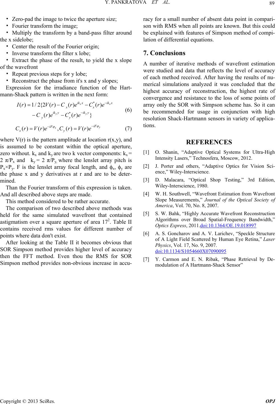

Y. PANKRATOVA ET AL.

• Zero-pad the image to twice the aperture size;

• Fourier transform the image;

• Multiply the transform by a band-pass filter around

the x sidelobe;

• Center the result of the Fourier origin;

• Inverse transform the filter x lobe;

• Extract the phase of the result, to yield the x slope

of the wavefront

• Repeat previous steps for y lobe;

• Reconstruct the phase from it's x and y slopes;

Expression for the irradiance function of the Hart-

mann-Shack pattern is written in the next form:

()1/2{2()()()

()()}

ik xik x

ik yik y

IrVrCreC re

Cre Cre





 (6)

() (),()()y

xiF

Cr VreCr Vre





 (7)

where V(r) is the pattern amplitude at location r(x,y), and

is assumed to be constant within the optical aperture,

zero without. kx and ky are two k vector components: kx =

2 π/Px and ky = 2 π/Py, where the lenslet array pitch is

Px×Py. F is the lenslet array focal length, and x, y are

the phase x and y derivatives at r and are to be deter-

mined.

Than the Fourier transform of this expression is taken.

And all described above steps are made.

This method considered to be rather accurate.

The comparison of two described above methods was

held for the same simulated wavefront that contained

astigmatism over a square aperture of area 172. Table II

contains received rms values for different number of

points where data don't exist.

After looking at the Table II it becomes obvious that

SOR Simpson method provides higher level of accuracy

then the FFT method. Even thou the RMS for SOR

Simpson method provides non-obvious increase in accu-

racy for a small number of absent data point in compari-

son with RMS when all points are known. But this could

be explained with features of Simpson method of compi-

lation of differential equations.

7. Conclusions

A number of iterative methods of wavefront estimation

were studied and data that reflects the level of accuracy

of each method received. After having the results of nu-

merical simulations analyzed it was concluded that the

highest accuracy of reconstruction, the highest rate of

convergence and resistance to the loss of some points of

array only the SOR with Simpson scheme has. So it can

be recommended for usage in conjunction with high

resolution Shack-Hartmann sensors in variety of applica-

tions.

REFERENCES

[1] O. Shanin, “Adaptive Optical Systems for Ultra-High

Intensity Lasers,” Technosfera, Moscow, 2012.

[2] J. Porter and others, “Adaptive Optics for Vision Sci-

ence,” Wiley-Interscience.

[3] D. Malacara, “Optical Shop Testing,” 3rd Edition,

Wiley-Interscience, 1980.

[4] W. H. Southwell, “Wavefront Estimation from Wavefront

Slope Measurements,” Journal of the Optical Society of

America, Vol. 70, No. 8, 2007.

[5] S. W. Bahk, “Highly Accurate Wavefront Reconstruction

Algorithms over Broad Spatial-Frequency Bandwidth,”

Optics Express, 2011.doi:10.1364/OE.19.018997

[6] A. S. Goncharov and A. V. Larichev, “Speckle Structure

of A Light Field Scattered by Human Eye Retina,” Laser

Physics, Vol. 17, No. 9, 2007.

doi:10.1134/S1054660X07090095

[7] Y. Carmon and E. N. Ribak, “Phase Retrieval by De-

modulation of A Hartmann-Shack Sensor”