Study on the Gain Material with Four Energy Level Model Using FDTD Method

doi:10.4236/opj.2013.32B004

Paper Menu >>

Journal Menu >>

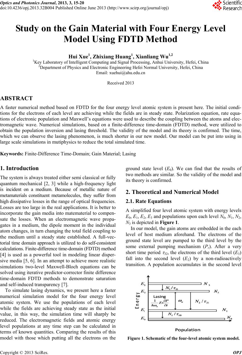Optics and Photonics Journal, 2013, 3, 15-20

doi:10.4236/opj.2013.32B004 Published Online June 2013 (http://www.scirp.org/journal/opj)

Study on the Gain Material with Four Energy Level

Model Using FDTD Method

Hui Xue1, Zhixiang Huang1, Xianliang Wu1,2

1Key Laboratory of Intelligent Computing and Signal Processing, Anhui University, Hefei, China

2Department of Physics and Electronic Engineering Hefei Normal University, Hefei, China

Email: [email protected]

Received 2013

ABSTRACT

A faster numerical method based on FDTD for the four energy level atomic system is present here. The initial condi-

tions for the electrons of each level are achieving while the fields are in steady state. Polarization equation, rate equa-

tions of electronic population and Maxwell’s equations were used to describe the coupling between the atoms and elec-

tromagnetic wave. Numerical simulations, based on a finite-difference time-domain (FDTD) method, were utilized to

obtain the population inversion and lasing threshold. The validity of the model and its theory is confirmed. The time,

which we can observe the lasing phenomenon, is much shorter in our new model. Our model can be put into using in

large scale simulations in mutiph ysics to reduce the total simulated time.

Keywords: Finite-Difference Time-Domain; Gain Material; Lasing

1. Introduction

The system is always treated either semi classical or fully

quantum mechanical [2, 3] while a high-frequency light

is incident on a medium. Because of metallic nature of

metamaterials constituent metamolecules, they suffer from

high dissipative losses in the range of optical frequencies.

Losses are too large in the real applications. It is better to

incorporate the ga in media into matematerial to compen-

sate the losses. When an electromagnetic wave propa-

gates in a medium, the dipole moment in the individual

atom changes, in turn changing the total field coupling to

the medium until a steady state established. A full-vec-

torial time domain approach is utilized to do self-consistent

calculations. Fin ite-difference time-domain (FDTD) method

[4] is used as a powerful tool in modeling linear disper-

sive media [5, 6]. In an attempt to achieve more realistic

simulations two-level Maxwell-Bloch equations can be

solved using iterative predictor-corrector finite difference

time-domain FDTD methods to demonstrate saturation

and self-induced transparency [7].

To simulate lasing dynamics, we present here a faster

numerical simulation model for the four energy level

atomic system. We use the populations of each level

while the fields are achieving steady state as the initial

value, in this way, the simulation time will sharply be

reduced. The electromagnetic fields and atomic energy

level populations at any time step can be calculated in

terms of known quantities. Comparing the results of this

model with those which putting all the electrons on the

ground state level (E0). We can find that the results of

two methods are similar. So the validity of the model and

its theory is confirmed.

2. Theoretical and Numerical Model

2.1. Rate Equations

A simplified four level atomic system with energy levels

E0, E1, E2, E3 and populations upon each level N0, N1, N2,

N3 is depicted in Figure 1.

In our model, the gain atoms are embedded in the each

level of host medium aforehand. The electrons of the

ground state level are pumped to the third level by the

some external pumping mechanism (Pr). After a very

short time period



32, the electrons of the third level (E3)

fall into the second level (E2) by a non-radioactively

transition. A population accumulates in the second level

Figure 1. Schematic of the four-level atomic system model.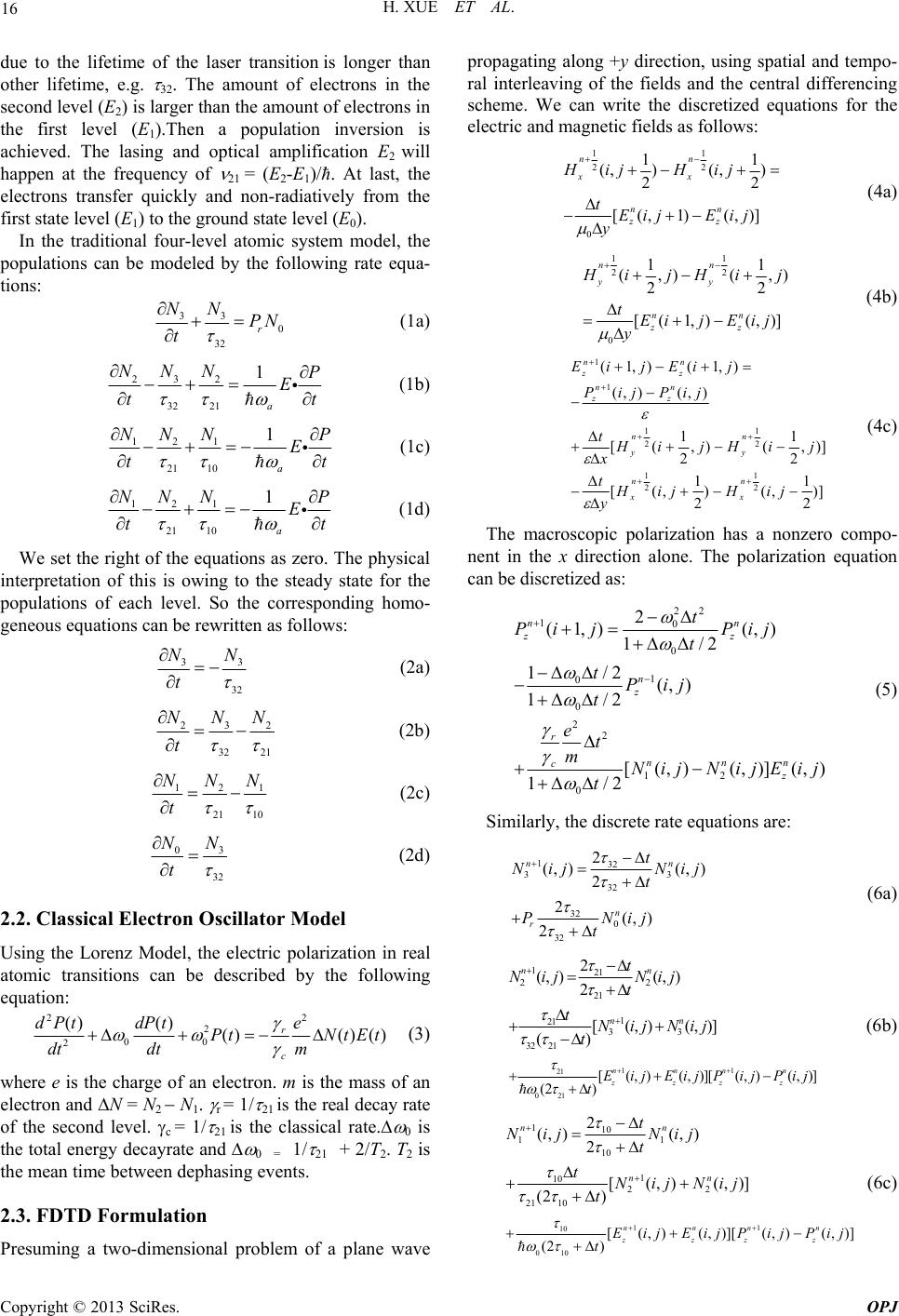

H. XUE ET AL.

due to the lifetime of the laser transition is longer than

other lifetime, e.g.



32. The amount of electrons in the

second level (E2) is larger than the amount of electrons in

the first level (E1).Then a population inversion is

achieved. The lasing and optical amplification E2 will

happen at the frequency of



21 = (E2-E1)/ħ. At last, the

electrons transfer quickly and non-radiatively from the

first state level (E1) to the ground state level (E0).

In the traditional four-level atomic system model, the

populations can be modeled by the following rate equa-

tions:

33 0

NNPN





 (1a)

32 21

NN P

 



 





 (1b)

121

21 10

NN NP

 









 (1c)

121

21 10

NN NP

 









t

(1d)

We set the right of the equations as zero. The physical

interpretation of this is owing to the steady state for the

populations of each level. So the corresponding homo-

geneous equations can be rewritten as follows:





 (2a)

32 21





 (2b)

21 10

NNN





 (2c)





 (2d)

2.2. Classical Electron Oscillator Model

Using the Lorenz Model, the electric polarization in real

atomic transitions can be described by the following

equation:

()() ()() ()

dPt dPte

Pt NtEt

dt mdt



 

  (3)

where e is the charge of an electron. m is the mass of an

electron and N = N2  N1.



r = 1/



21 is the real decay rate

of the second level. c = 1/



21 is the classical rate.



0 is

the total energy decayrate and 



0 = 1/



21 + 2/T2. T2 is

the mean time between dephasing events.

2.3. FDTD Formulation

Presuming a two-dimensional problem of a plane wave

propagating along +y direction, using spatial and tempo-

ral interleaving of the fields and the central differencing

scheme. We can write the discretized equations for the

electric and magnetic fields as follows:

(, )(, )

[(, 1)(,)]

Hij Hij

tEij Eij

















(4a)

(,) (,

[(1,) (,)]

Hi jHi j

tEij Eij





 







)

(4b)

(1,)(1,)

(, )(, )

[(,) (,

[(,) (,)

Ei jEi j

PijPij

tHi jHi j

tHij Hij







 













)]

]

(4c)

The macroscopic polarization has a nonzero compo-

nent in the x direction alone. The polarization equation

can be discretized as:

(1,) (,)

1/2

(, )

1/2

[(, )(, )](, )

1/2

nnn

Pi jPij

tPij

mNij NijEij















 

 

 





 

(5)

Similarly, the discrete rate equations are:

132

32 0

(, )(, )

2(, )

ijN ij

PNij









(6a)

021

121

21 33

32 21

[ (,)(,)][ (,)(,)]

(2 )

(, )(, )

[(,) (,)]

()

nnnn

zzzz

EijE ijPijPij

Nij Nij

tNijNij





























(6b)

010

110

10 22

21 10

[(, )(, )][(, )(,)]

(2 )

(, )(,)

[(,)(,)]

(2 )

nnnn

zzzz

EijE ijPijP ij

Nij Nij

tNijNij





























(6c)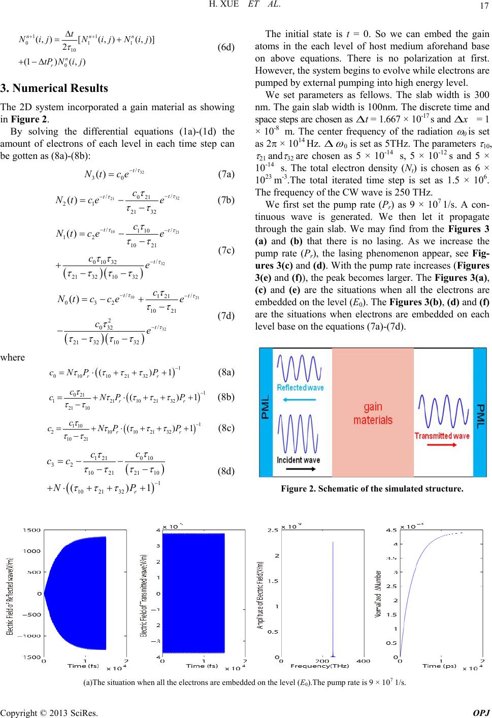

H. XUE ET AL.

The initial state is t = 0. So we can embed the gain

atoms in the each level of host medium aforehand base

on above equations. There is no polarization at first.

However, the system begins to evolve while electrons are

pumped by exte rnal p umping into hig h energy level.

(, )[(, )(, )]

(1)( ,)

ijNijN ij

tPNij











(6d)

3. Numerical Results We set parameters as fellows. The slab width is 300

nm. The gain slab width is 100nm. The discrete time and

space s teps are chosen a s ∆t = 1.667 × 10-17 s and ∆x = 1

× 10-8 m. The center frequency of the radiation



0 is set

as 2 × 1014 Hz. ∆

0 is set as 5THz. The p arameters



10,



21 and



32 are chosen as 5 × 10-14 s, 5 × 10-12 s and 5 ×

10-14 s. The total electron density (Nt) is chosen as 6 ×

1023 m-3.The total iterated time step is set as 1.5 × 106.

The frequency of the CW wave is 250 THz.

The 2D system incorporated a gain material as showing

in Figure 2.

By solving the differential equations (1a)-(1d) the

amount of electrons of each level in each time step can

be gotten as (8a)-(8b):

() t

Nt ce





 (7a)

21 /

/021

21 32

() t

Nt cee









 (7b) We first set the pump rate (Pr) as 9 × 107 1/s. A con-

tinuous wave is generated. We then let it propagate

through the gain slab. We may find from the Figures 3

(a) and (b) that there is no lasing. As we increase the

pump rate (Pr), the lasing phenomenon appear, see Fig-

ures 3(c) and (d). With the pump rate increases (Figures

3(e) and (f)), th e peak be comes larg er. The Figures 3(a),

embedded on the level (E0). The Figures 3(b), (d) and (f)

are the situations when electrons are embedded on each

level base on the equations (7a)-(7d).



10 21

110

10 21

010 32

21 32 1032

() tt

Nt cee

















(7c)



10 21

121

032

10 21

032

21 32 1032

() tt

Ntc cee













 



(7d)

where



010 102132

()

cNP P





1

(8a)



021

121102132

21 10

()

cNP P









 (8b)



110

210102132

10 21

()

cNPP









 (8c)



010

121

102121 10

1021 32

()

NP1







 



 

(8d)

Figure 2. Schematic of the simulated structure.

(a)The situation when all the electrons are embedded on the level (E0).The pump rate is 9 × 107 1/s.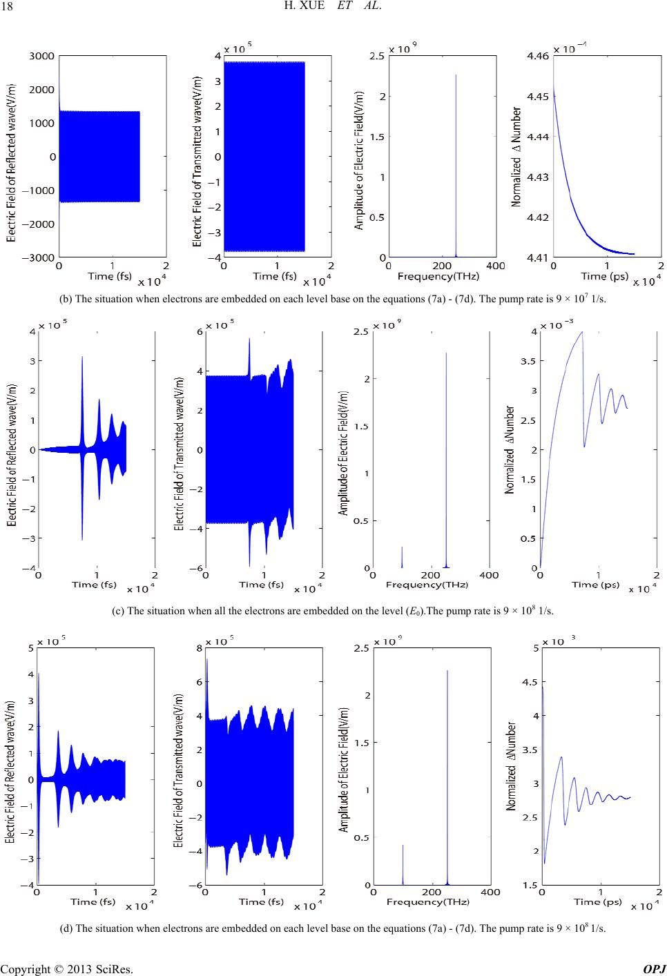

H. XUE ET AL.

(b) The situation when electrons are embedded on each level base on the equations (7a) - (7d). The pump rate is 9 × 107 1/s.

(d) The situation when electrons are embedded on each level base on the equations (7a) - (7d). The pump rate is 9 × 108 1/s.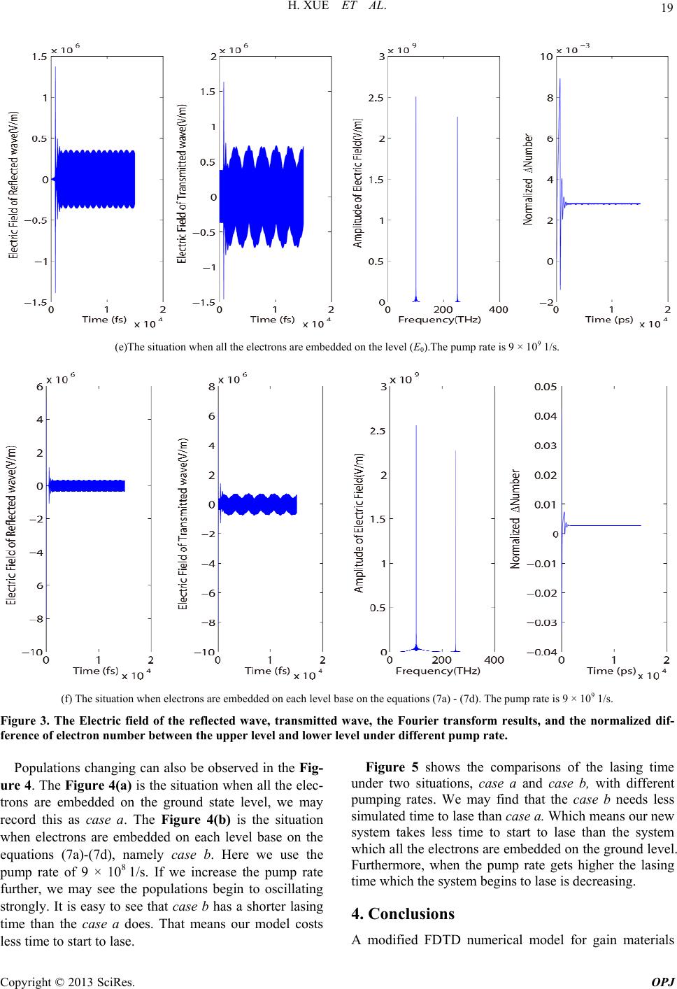

H. XUE ET AL.

(e)The situation when all the electrons are embedded on the level (E0).The pump rate is 9 × 109 1/s.

(f) The situation when electrons are embedded on each level base on the equations (7a) - (7d). The pump rate is 9 × 109 1/s.

Figure 3. The Electric field of the reflected wave, transmitted wave, the Fourier transform results, and the normalized dif-

ference of electron number between the upper level and lower level under different pump rate.

Populations changing can also be observed in the Fig-

ure 4. The Figure 4(a) is the situation when all the elec-

trons are embedded on the ground state level, we may

record this as case a. The Figure 4(b) is the situation

when electrons are embedded on each level base on the

equations (7a)-(7d), namely case b. Here we use the

pump rate of 9 × 108 1/s. If we increase the pump rate

further, we may see the populations begin to oscillating

strongly. It is easy to see that case b has a shorter lasing

time than the case a does. That means our model costs

Figure 5 shows the c

less time to start to lase.

omparisons of the lasing time

4. Conclusions

umerical model for gain materials

der two situations, case a and case b, with different

pumping rates. We may find that the case b needs less

simulated time to lase than case a. Which means our new

system takes less time to start to lase than the system

which all the electrons are embedded on the ground level.

Furthermore, when the pump rate gets higher the lasing

time which the system begins to lase is decreasing.

A modified FDTD n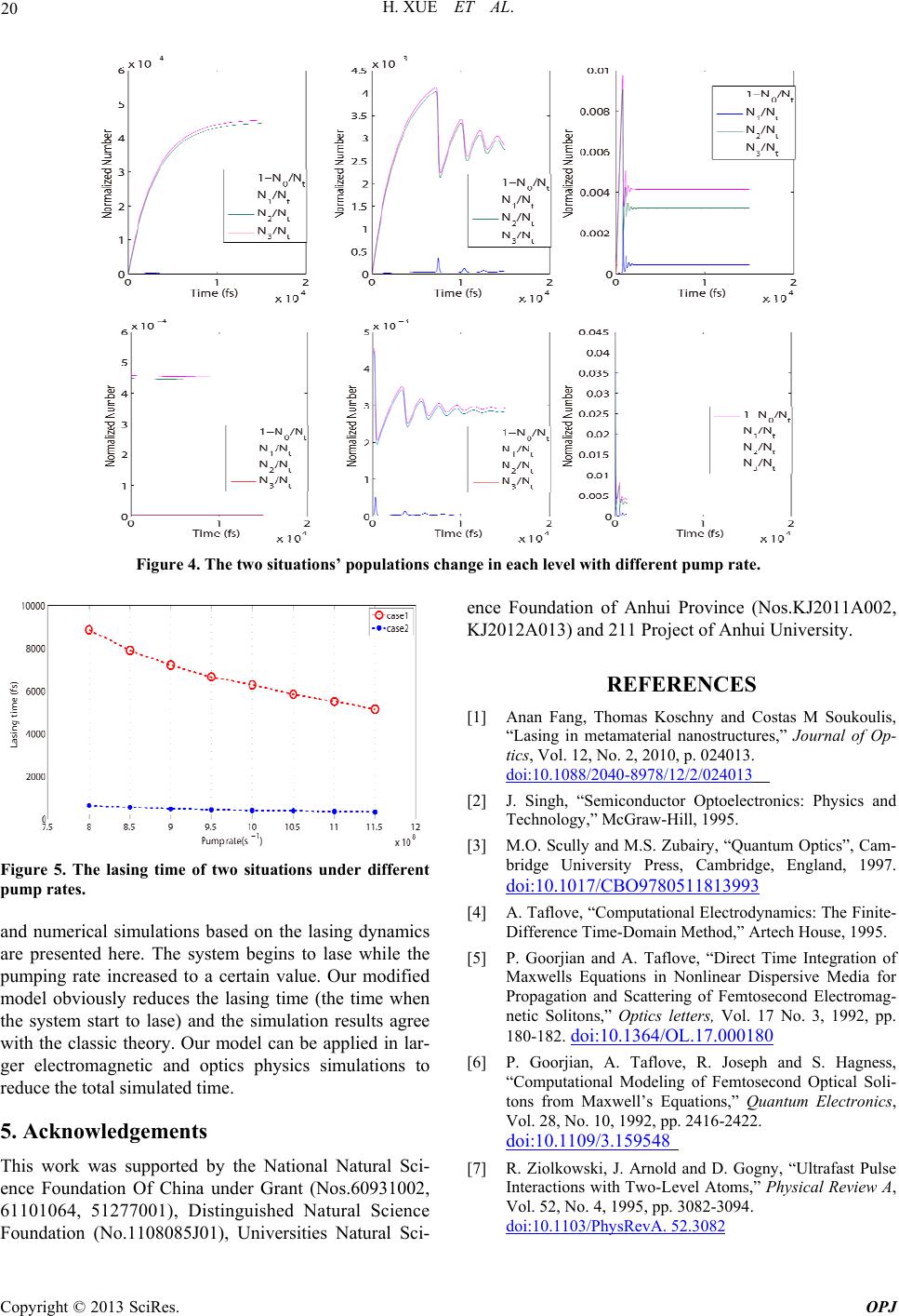

H. XUE ET AL.

Figure 4. The two situations’ populations change in each level with different pump rate.

Figure 5. The lasing time of two situations under differen

nd numerical simulations based on the lasing dynamics

5. Acknowledgements

the National Natural Sci-

ence Foundation of Anhui Province (Nos.KJ2011A002,

[1] Anan Fang, Tstas M Soukoulis,

“Lasing in mes,” Journal of Op-

pump rates.

are presented here. The system begins to lase while the

pumping rate increased to a certain value. Our modified

model obviously reduces the lasing time (the time when

the system start to lase) and the simulation results agree

with the classic theory. Our model can be applied in lar-

ger electromagnetic and optics physics simulations to

reduce the total simulated time.

This work was supported by

ence Foundation Of China under Grant (Nos.60931002,

61101064, 51277001), Distinguished Natural Science

Foundation (No.1108085J01), Universities Natural Sci-

KJ2012A013) and 211 Project of Anhui University.

REFERENCES

homas Koschny and Co

tamaterial nanostructure

tics, Vol. 12, No. 2, 2010, p. 024013.

doi:10.1088/2040-8978/12/2/024013

[2] J. Singh, “Semiconductor Optoelectr

Technology,” McGraw-Hill, 1995. onics: Physics and

ge, England, 1997.

[3] M.O. Scully and M.S. Zubairy, “Quantum Optics”, Cam-

bridge University Press, Cambrid

doi:10.1017/CBO9780511813993

[4] A. Taflove, “Computational Electrodynamics: The Finite-

Difference Time-Domai n Method,” Artech House, 1995.

[5] P. Goorjian and A. Taflove, “Direct Time Integration of

Maxwells Equations in Nonlinear Dispersive Media for

Propagation and Scattering of Femtosecond Electromag-

netic Solitons,” Optics letters, Vol. 17 No. 3, 1992, pp.

180-182. doi:10.1364/OL.1 7.000180

[6] P. Goorjian, A. Taflove, R. Joseph and S. Hagness,

“Computational Modeling of Femtosecond Optical Soli-

tons from Maxwell’s Equations,” Quantum Electronics,

Vol. 28, No. 10, 1992, pp. 2416-2422.

doi:10.1109/3.159548

[7] R. Ziolkowski, J. Arnold and D. Gogn

Interactions with Two-Levy, “Ultrafast Pulse

el Atoms,” Physical Review A,

Vol. 52, No. 4, 1995, pp. 3082-3094.

doi:10.1103/PhysRevA. 52.3082