

Paper Menu >>
Journal Menu >>
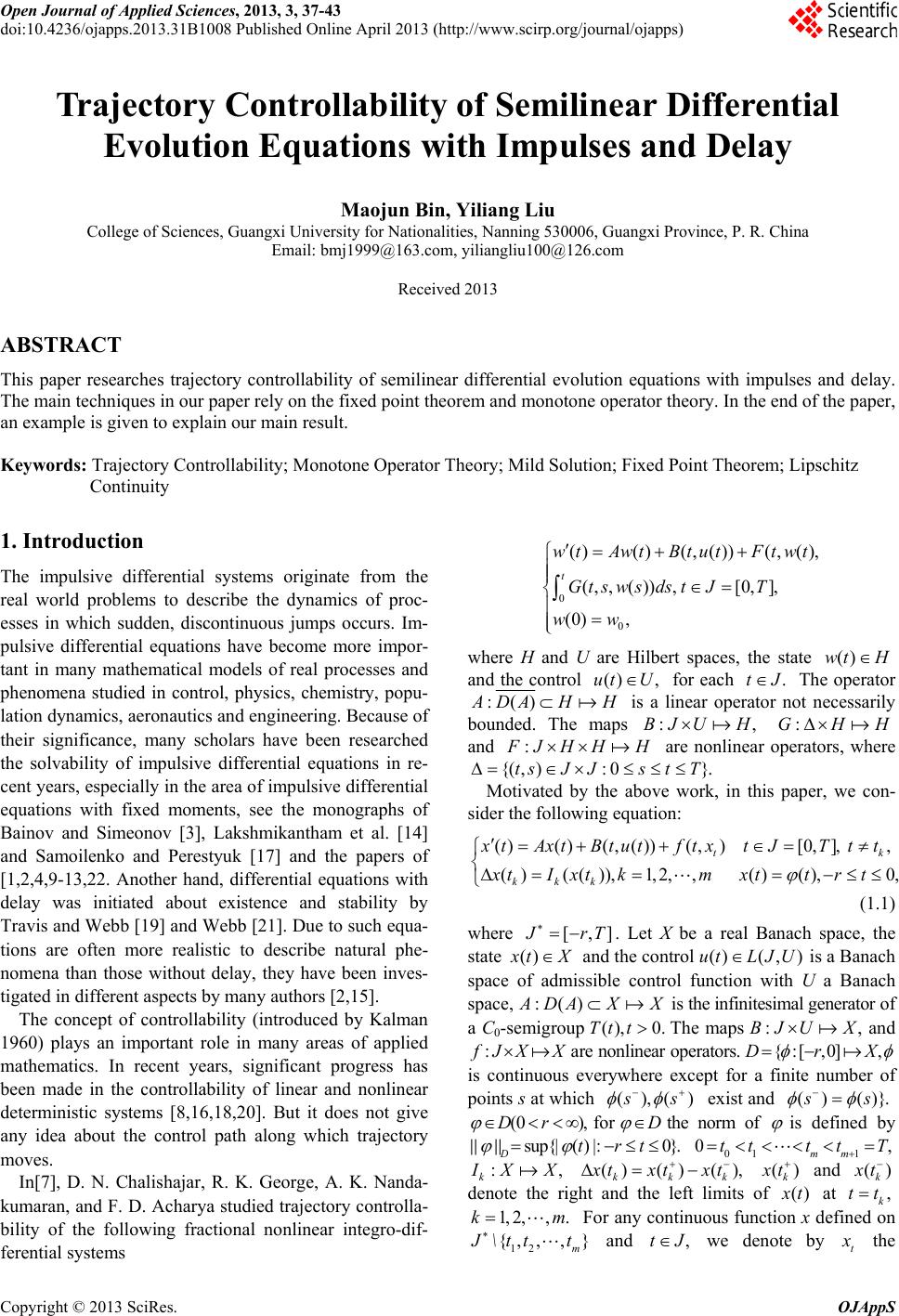 Open Journal of Applied Sciences, 2013, 3, 37-43 doi:10.4236/ojapps.2013.31B1008 Published Online April 2013 (http://www.scirp.org/journal/ojapps) Trajectory Controllability of Semilinear Differential Evolution Equations with Impulses and Delay Maojun Bin, Yiliang Liu College of Sciences, Guangxi University for Nationalities, Nanning 530006, Guangxi Province, P. R. China Email: [email protected], [email protected] Received 2013 ABSTRACT This paper researches trajectory controllability of semilinear differential evolution equations with impulses and delay. The main techniques in our paper rely on the fixed point theorem and monotone operator theory. In the end of the paper, an example is given to explain our main result. Keywords: Trajectory Controllability; Monotone Operator Theory; Mild Solution; Fixed Point Theorem; Lipschitz Continuity 1. Introduction The impulsive differential systems originate from the real world problems to describe the dynamics of proc- esses in which sudden, discontinuous jumps occurs. Im- pulsive differential equations have become more impor- tant in many mathematical models of real processes and phenomena studied in control, physics, chemistry, popu- lation dynamics, aeronautics and engineering. Because of their significance, many scholars have been researched the solvability of impulsive differential equations in re- cent years, especially in the area of impulsive differential equations with fixed moments, see the monographs of Bainov and Simeonov [3], Lakshmikantham et al. [14] and Samoilenko and Perestyuk [17] and the papers of [1,2,4,9-13,22. Another hand, differential equations with delay was initiated about existence and stability by Travis and Webb [19] and Webb [21]. Due to such equa- tions are often more realistic to describe natural phe- nomena than those without delay, they have been inves- tigated in different aspects by many authors [2,15]. The concept of controllability (introduced by Kalman 1960) plays an important role in many areas of applied mathematics. In recent years, significant progress has been made in the controllability of linear and nonlinear deterministic systems [8,16,18,20]. But it does not give any idea about the control path along which trajectory moves. In[7], D. N. Chalishajar, R. K. George, A. K. Nanda- kumaran, and F. D. Acharya studied trajectory controlla- bility of the following fractional nonlinear integro-dif- ferential systems 0 0 ()()( ())(() (()) [0] (0) t wtAwt BtutFtwt Gtsws dstJT ww where H and U are Hilbert spaces, the state ()wt H and the control ()ut U for each The operator tJ () A DA HHBJ H is a linear operator not necessarily bounded. The maps and U HGH F JHH {( )ts JH 0J s are nonlinear operators, where }t T Motivated by the above work, in this paper, we con- sider the following equation: ()()(())()[0] ( )(( ))12()()0 tk kkk x tAxtBtut ftxtJTtt xtI xtkmxttrt (1.1) where [] J rT () . Let X be a real Banach space, the state x tX and the control is a Banach space of admissible control function with U a Banach space, () ()ut LJU () A DA X ()TtX 0t is the infinitesimal generator of a C0-semigroup The maps and BJUX f JX X are nonlinear operators. {[Dr0] X ) is continuous everywhere except for a finite number of points s at which ()( s s exist and () ()} s s (0 )Dr for D the norm of is defined by sup{( )tr0}t D 01 tt 0mm k 1 tt T I XX kkk ()() () x txtxt () k x t and () k x t denote the right and the left limits of () x t at k tt 12km 12 {} m For any continuous function x defined on J \tt t and tJ we denote by t x the Copyright © 2013 SciRes. OJAppS 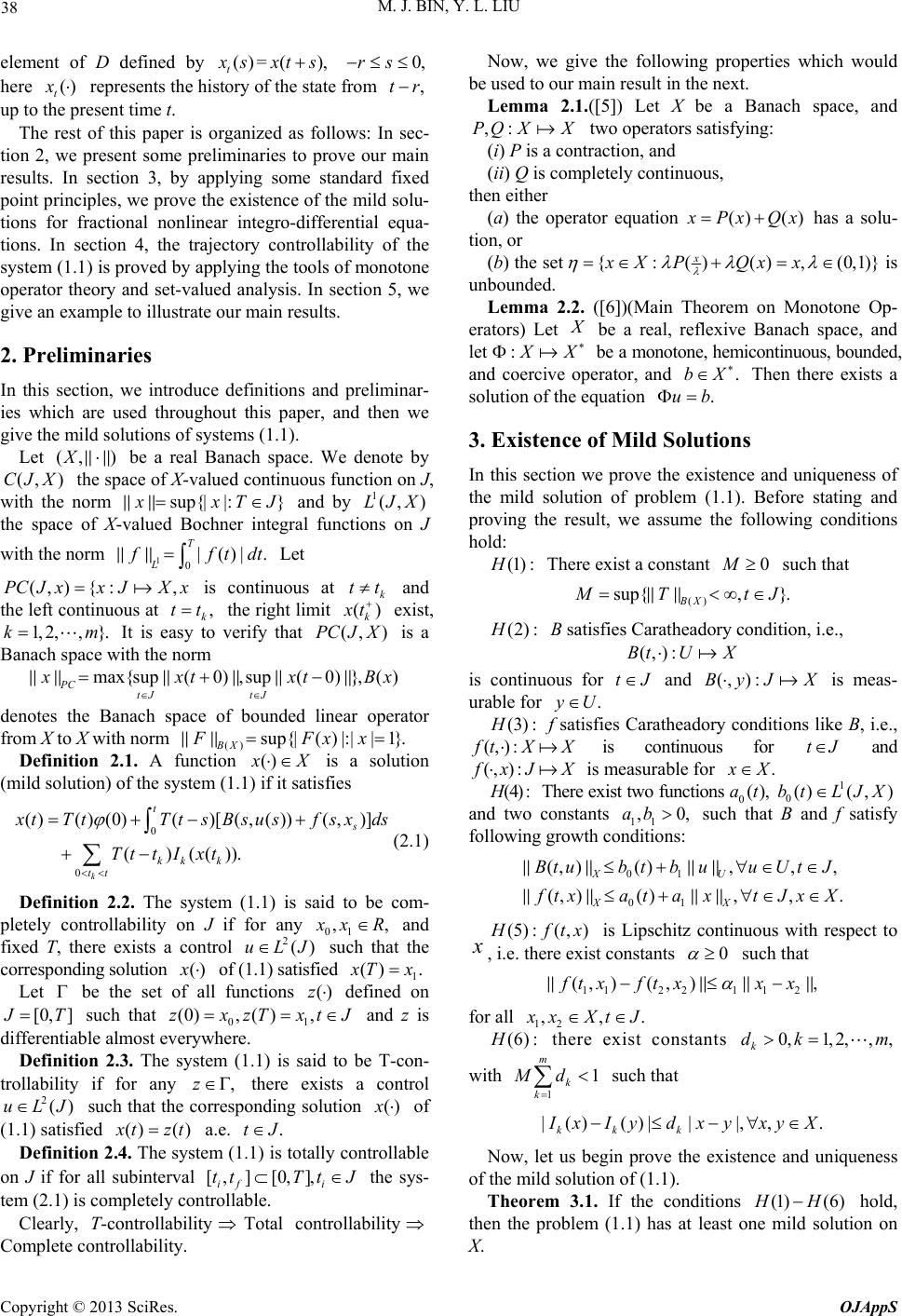 M. J. BIN, Y. L. LIU 38 element of D defined by ()= () t x sxts here 0rs () t x represents the history of the state from tr the present time t. up to ) The rest of this paper is organized as follows: In sec- tion 2, we present some preliminaries to prove our main results. In section 3, by applying some standard fixed point principles, we prove the existence of the mild solu- tions for fractional nonlinear integro-differential equa- tions. In section 4, the trajectory controllability of the system (1.1) is proved by applying the tools of monotone operator theory and set-valued analysis. In section 5, we give an example to illustrate our main results. 2. Preliminaries In this section, we introduce definitions and preliminar- ies which are used throughout this paper, and then we give the mild solutions of systems (1.1). Let be a real Banach space. We denote by the space of X-valued continuous function on J, with the norm (X () X CJ sup{ } x xT J and by 1()LJX the space of X-valued Bochner integral functions on J with the norm 10 T L() f ft dt Let ()Jx{PCxJX x is continuous at k tt and the left continuous at k the right limit tt() k x t exist, It is easy to verify that 12k }m ()J XPC is a Banach space with the norm max{sup( tJ 0)sup( tJ 0)}() PC x xtxt sup{( )FF Bx 1}xx denotes the Banach space of bounded linear operator from X to X with norm ()BX () Definition 2.1. A function x X )[(())( )) k is a solution (mild solution) of the system (1.1) if it satisfies 0 () (0)( ()(( k t kk tt 0 () )] s x tTt Tt Ttt Ix sBsusf t sxds (2.1) Definition 2.2. The system (1.1) is said to be com- pletely controllability on J if for any 01 x xR and fixed T, there exists a control such that the corresponding solution 2()uLJ () x of (1.1) satisfied 1 () x Tx Let be the set of all functions defined on [0 ] ()z J T 2()J such that 0 and z is differentiable almost everywhere. 1 tJ () (0)( )zx zTx Definition 2.3. The system (1.1) is said to be T-con- trollability if for any there exists a control such that the corresponding solution z uL x of (1.1) satisfied ()() x tzt a.e. tJ [][0] if i tt Tt Definition 2.4. The system (1.1) is totally controllable on J if for all subinterval J the sys- tem (2.1) is completely controllable. Clearly, T-controllability Total controllability Complete controllability. Now, we give the following properties which would be used to our main result in the next. Lemma 2.1.([5]) Let X be a Banach space, and PQ XX two operators satisfying: (i) P is a contraction, and (ii) Q is completely continuous, then either (a) the operator equation ()() x Px Qx has a solu- tion, or (b) the set {()()(0 x xX PQx x 1)} is unbounded. Lemma 2.2. ([6])(Main Theorem on Monotone Op- erators) Let be a real, reflexive Banach space, and let X X X be a monotone, hemicontinuous, bounded, and coercive operator, and Then there exists a solution of the equation bX ub 3. Existence of Mild Solutions In this section we prove the existence and uniqueness of the mild solution of problem (1.1). Before stating and proving the result, we assume the following conditions hold: (1)H There exist a constant such that 0M () sup{ } BX M TtJ (2)H B satisfies Caratheadory condition, i.e., ()Bt UX is continuous for tJ and is meas- urable for ()ByJ X y U (3)H () f satisfies Caratheadory conditions like B, i.e., f tXX is continuous for tJ and () f xJ X is measurable for x X ()at (4)H There exist two functions 0 0 1 ()bt L()JX and two constants 11 0ab such that B and f satisfy following growth conditions: 01 01 () () () () XU XX Btub tbuuUtJ f txataxtJxX (5)( ) H ftx is Lipschitz continuous with respect to x , i.e. there exist constants 0 such that 112 2112 ()( ) f txftxxx for all 12 x xXtJ ) (6H m there exist constants 012 k dk m with 1 1 k k Md such that () () kk k I xIydxy xyX Now, let us begin prove the existence and uniqueness of the mild solution of (1.1). Theorem 3.1. If the conditions hold, then the problem (1.1) has at least one mild solution on X. (1) (6)HH Copyright © 2013 SciRes. OJAppS 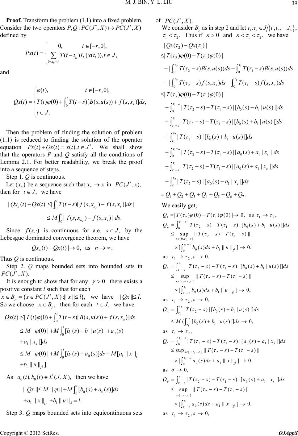 M. J. BIN, Y. L. LIU 39 Proof. Transform the problem (1.1) into a fixed problem. Consider the two operators defined by () ()PQPCJXPCJX 0 0[0] () ()(()) k kk k tt tr Px tTtt IxttJ and 0 ()[ 0] ()()(0)()[(())()] t s ttr QxtT tTtsBsusfsxds tJ Then the problem of finding the solution of problem (1.1) is reduced to finding the solution of the operator equation We shall show that the operators P and Q satisfy all the conditions of Lemma 2.1. For better readability, we break the proof into a sequence of steps. ()() ()PxtQxtxttJ Step 1. Q is continuous. Let {} n x be a sequence such that n x x in ()PC Jx then for we have tJ 0 0 ()()()[()()] ()() s s t nn t ns QxtQxtT tsfs xfs xds Mfsxfsxds s Since () f s is continuous for a.e. s J by the Lebesgue dominated convergence theorem, we have ()()0, as . n QxtQxtn Thus Q is continuous. Step 2. Q maps bounded sets into bounded sets in ()PCJX It is enough to show that for any 0 } there exists a positive constant l such that for each {() x BxPCJXxl we have Qx l So we choose x B then for each we have tJ 1 1 0 01 0 0 1 00 1 0 1 ( )( )(0)()[(())()] (0)[ ()()() ] (0)[ ()()][ ] t s t s t L L Qx tTtTtsBs usfsxds MMbsbusas axds M MbsasdsMax bu As then we have 1 00 () ()()atbt LJX 11 00 0 11 [()()] t LL QxMMbsas ds ax bu l Step 3. Q maps bounded sets into equicontinuous sets of ()PC JX We consider B as in step 2 and let 1212m J tt t 12 Thus if 0 and 12 we have 21 21 1 21 21 21 00 21 00 21 2101 0 ()() ()(0) ()(0) ()(())()(()) ()()()() ()(0) ()(0)| ()()[()()] ss Qx Qx TT TsBsusdsTsBsus ds TsfsxdsTsfsxds TT TsTsbsbusds 1 1 2 1 1 1 1 2 1 2101 201 2101 0 2101 201 ()()[()()] ()[()()] ()()[()] ()()[()] ()[()] s s s TsTsbsbusds Tsbsbusds TsTsasaxds TsTsasaxds Tsasaxds Q 1234567 QQQQQQ We easily get, 1 1 1 1 1 1 12 112 22101 0 21 [0 ] 01 0 12 3210 ()(0)()(0)0 as ()()[()()] sup()() [()]0 as 0 ()()[() s L QT T QTsTsbsbus TsTs bsdsb u QTsTsbsb ds 11 1 1 1 2 1 2 1 1 1 21 [] 01 12 4201 01 12 521 0 ()] sup()() [()]0 as 0 ()[() ()] ([()()]0 as ()()[ s L us ds TsTs bsdsb u QTsbsbusds Mbsbusds QTsTs 1 1 1 1 1 [] 11 1 1 01 [0 ]21 01 0 62101 21 01 () ] sup()() [()]0 as 0 ()()[()] sup()() [() s s s L s asa xds TsTs asdsa x QTsTsasaxd TsTs asdsa x 1 12 ]0 as 0 L s Copyright © 2013 SciRes. OJAppS 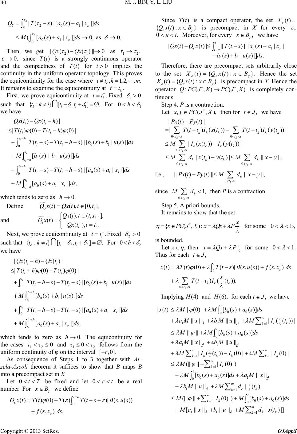 M. J. BIN, Y. L. LIU 40 2 1 2 1 7201 01 ()[() ] ([()]0 as 0 s s QTsasaxds Masaxds Then, we get 21 ()() 0Qx Qx as 12 0 since is a strongly continuous operator and the compactness of for implies the continuity in the uniform operator topology. This proves the equicontinuity for the case where k It remains to examine the equicontinuity at () ()Tt0t tt tt Tt 12 m t 0 k tk First, we prove equicontinuity at Fixed i1 such that For 11 {}[ kii tki tt ] 1 0h we have 01 0 01 01 0 01 ()() ()(0) ()(0) ()()[()()] [()()] ()()[()] [()] i i i i i i ii ii th ii t th th ii s t s th Qx tQx th TtTth TtsTthsb sb usds Mbsbusds TtsTthsa saxds Masaxds which tends to zero as 0h D efine 01 ()()[0 ]QxtQxttt and 1 () (] () () ii iii Qx tttt QxtQx ttt Next, we prove equicontinuity at Fixed i tt 20 h such that For 22 {}[ kii tki tt ] 2 0 we have 01 0 01 01 0 01 ()() ()(0)()(0) ()()[()() [()()] ()()[()] [()] i i i i i i ii ii t ii th t t ii s th s t Qx thQx t Tt hTt Tt hsTtsbsbusds Mbsbusds Tt hsTts as axds Masaxds ] which tends to zero as The equicontnuity for the cases 12 0h 0 and 12 0 follows from the uniform continuity of φ on the interval [0]r As consequence of Steps 1 to 3 together with Ar- zela-Ascoli theorem it suffices to show that B maps B into a precompact set in X. Let be fixed and let 0tT 0t be a real number. For x B we define 0 ()()(0)()()[(()) ()] t s QxtTtTTt sBsus fsx ds Since is a compact operator, the set ()Tt () X t {(Qxt)x B} is precompact in X for every 0t Moreover, for every x B we have 01 01 ()()()[() ()()] t s t Qx tQx tTtsasax bsbus ds Therefore, there are precompact sets arbitrarily close to the set () {()} X tQxtxB () } Hence the set () { X tQxtxB () ()QPCJ XPCJ X is precompact in X. Hence the operator is completely con- tinuous. Step 4. P is a contraction. Let () x yPCJX then for t we have J 00 0 00 ()() ()(()) ()(()) ( ())(()) () () kk k kk kk kkkk tt tt kk kk tt kk kk tt tt Px tPy t TttIxt TttIyt MIxtIyt MdxtytMdxy i.e., 0 () () k k tt Px tPytMdxy since 0 1 k k tt Md then P is a contraction. Step 5. A priori bounds. It remains to show that the set {() x x PC JXxQxP for some 01} is bounded. Let x then x x Qx P for some 01 Thus for each tJ 0 0 ()()(0)()[(())()] ()(()) k t s kk k tt x tTt TtsBsusfsxd x Ttt It s Implying and for each we have (4)H(6)HtJ 11 11 00 0 11 1 00 0 11 11 ()(0)[( )( )] (()) [()()] (())(0)(0) t mx kk k LL t LL mm x kk kk kk xtMMbsas ds aMxbM uMIt MMbsasds aMxbM u MItI MI 1 1 11 1 001 0 11 00 10 11 1 ((0)) [()()] () ((0))[()()] [()] m k k t L mx kk k Lt m k k m kk k LL MI Mbsasds aMx bM uMdt M IMbsasd Maxb uMdxt s Copyright © 2013 SciRes. OJAppS  M. J. BIN, Y. L. LIU 41 Now we consider the function defined by ()sup{()}0txsrsttT Then () s x t for all tJ and there is a point such that If by the previous inequality we have for note [t ]rt() (J ( )txt ttJ tt 11 00 10 11 1 ()((0))[ ()()] [()] t m k k m k k LL tMIMbsasds Maxb uMdt i.e., 11 1 1 00 0 11 (1)()((0) ) [()()] [] mm kk k k t LL Md tMI M bs asds Maxbu Hence there exists a constant K such that, 1 11 1 1 1 00 0 11 () ((0)) [()()] [] mk k m k k Md T LL t{M I Mbsasds Maxb u} K By the definition of we have sup()() tJ xxtTKx This shows that the set is bounded. As a conse- quence of Theorem 3.1 we deduce that has a fixed point which is a mild solution of problem (1.1). PQ The proof is completed. 4. T-Controllability Results In this section, we are concerned with the trajectory con- trollability of semilinear differential evolution equations with impulses and delay. We make the following additional assumption on B: H(7): B satisfies monotonicity and coercivity condi- tions, i.e., () ()0BtuBtv uvuvUtJ and () lim u Btu u u Now let begin proving the T-controllability results for the problem (1.1). Theorem 4.1. Under the conditions the problem (1.1) is T-controllable. (1) (7)HH Proof. Let be the prescribed trajectory with zT (0)(0) z we want to find a control u satisfying 0 0 ()()(0)()[(())()] ()(()) k t s kk k tt ztTtTtsBsusf szds Ttt Izt (4.1) The equation (4.1) can be written as 0 0 0 ()()(0)()() ()(()) ()(()) k t s kk k tt t ztTtTtsfszds TttIzt TtsBsus ds (4.2) Differentiating with respect to t, we get 0 0 0 ()()(0)()()() ()(()) ()(())(( )) k t s t kk k tt t ztATtATt sfszdsftz ATttIzt ATtsBs usdsB tut - (4.3) Equation (4.3) can be written as 0 0 ()()()() t ytgtsysdsy t (4.4) where ()(()) ()()ytBtutgtsATt s and 0 0 0 ()()() (0) ()()() ()(()) k t s t kk k tt ytzt ATt A Ttsfszdsftz ATttIz t Define an operator by 22 () (LJX LJX t ) 0 ()()( )yt gtsysds (4.5) We easily know that 0 is continuous in ()yt () J gts is continuous in J J then for any 2() 12 y yLJX we have 0 12 12 00 12 0 12 ()()()() max()( )( ) tT tt T yy g tsy sdsgtsysds g tsy sysds Ly y = n is a contraction for sufficiently large n. Hence by generalized Banach contraction principle, there exists a unique solution y for (4.4) for given 2 0() y LJX Therefore, T-controllability follows if we can extract from the relation ()ut ()(())yt Btut ) (4.6) To see this, define an operator by 22 () (NLJXLJX ( ())t ut ()NutB (4.7) By the conditions H(1) and H(4), N is well-defined, continuous and bounded operator. Also, (())Btut is monotone and coercive, then we can easily get N is monotone and coercive. A hemi-continuous monotone mapping is of type (M). The nonlinear map N is onto. By Lemma 2.2, there exists a control u satisfying (4.6). The measurability of follows as u is in ()ut2()LJX This proves T- controllability of the problem (1.1). Copyright © 2013 SciRes. OJAppS  M. J. BIN, Y. L. LIU 42 The proof is completed. 5. Application Example. We consider the following semilinear impul- sive equation: 2 1 ()() [cos()cos()] 3 [0] (0)(0)1 2 () () ()() (()) k kkkk wtxw utxxtwt ttJ Ttt wx xinkm wtxtx inJ wtxwtxI wtx (5.1) where is abounded domain in with smooth boundary (1 n Rn ( )L ) 2 (0 )()xtx 2()XL We take and define the operator () A DAX X by 21 0 ()()() ()DA HHAwAxDw It is easily turned out that the operator A generates equicontinuous -semigroup on X. re the control term is linear, 0 C )(()) (Btut ut 2 1 () [cos()cos() 3 t] f txxt wt is Lipchitz conditions. It satisfies the conditions of Theorem 4.1, then the problem (5.1) is T-controllable. 6. Acknowledgements This work was financially supported by NNSF of China Grant No.11271087, No.61263006, Guangxi Scientific Experimental (China- ASEAN Research) Centre No. 20 120116, open fund of Guangxi Key laboratory of hybrid computation and IC design analysis No.2012HC IC07, and the Innovation Project of Guangxi Graduate Educa- tion No. YCSZ2012062. REFERENCES [1] A. Anguraj and M. Mallika Arjunan, “Existence and Uniqueness of Mild and Classical Solutions of Impulsive Evolution Equations,” Electronic Journal of Differential Equations, Vol. 111, 2005, pp. 1-8. [2] A. Anguraj and M. Mallika Arjunan, “Existence Results for an Impulsive Neutral Integro-differential Equations in Banach Spaces,” Nonlinear Study, Vol. 16, No. 1, 2009, pp. 33-48. [3] D. D. Bainov and P. S. Simeonov, “Impulsive Differen- tial Equations: Periodic Solutions and Applications,” Longman Scientific and Technical Group, England, 1993. [4] M. Benchohra J. Henderson and S. K. Ntouyas, “Exis- tence Results for Impulsive Multivalued Semilinear Neu- tral Functional Inclusions in Banach Spaces,” Journal of Mathematical Analysis and Applications, Vol. 263, No. 2, 2001, pp. 763-780. doi:10.1006/jmaa.2001.7663 [5] T. A. Burton and Colleen Kirk, “A Fixed Point Theorem of Krasnoselskiii-Schaefer Type,” Mathematische Nachrichten, Vol. 189, No. 1, 1998, pp. 23-31. doi:10.1002/mana.19981890103 [6] S. Carl and S. Heikkila, “Fixed Point Theory in Ordered Sets and Applications,” Springer, New York, Dordrecht, Heidelberg, London, 2010. [7] D. N. Chalishajar, R. K. George, A. K. Nandakumaran and F. S. Acharya, “Trajectory Controllability of Nonlin- ear Integro-differential System,” Journal of Frankin In- situte., Vol. 347, No. 7, 2010, pp. 1065-1075. doi:10.1016/j.jfranklin.2010.03.014 [8] L. Chen and G. Li, “Approximate Controllability of Im- pulsive Differential Equations with Nonlocal Condi- tions,” International Journal of Nonlinear Science, Vol. 10, 2010, pp. 438-446. [9] Z. Fan, “Impulsive Problems for Semilinear Differential Equations with Nonlocal Conditions,” Nonlinear Analysis, Vol. 72, No. 2, 2010, pp. 1104-1109. doi:10.1016/j.na.2009.07.049 [10] Z. Fan and G. Li, “Existence Results for Semilinear Dif- ferential Equations with Nonlocal and Impulsive Condi- tions,” Journal of Functional Analysis, Vol. 258, No. 5, 2010, pp. 1709-1727. doi:10.1016/j.jfa.2009.10.023 [11] E. Hernandez, M. Pierri and G. Goncalves, “Existence Results for an Impulsive Abstract Partial Differential Equation with State-dependent Delay,” Computer Math- ematic Application, Vol. 52, No. 3-4, 2006, pp. 411-420. doi:10.1016/j.camwa.2006.03.022 [12] E. Hernandez, M. M. Rabello and H. Henriaquez, “Exis- tence of Solutions for Impulsive Partial Neutral Func- tional Differential Equations,” Journal of Mathematic Analysis and Application, Vol. 331, No. 2, 2007, pp. 1135-1158. doi:10.1016/j.jmaa.2006.09.043 [13] S. Ji and S. Wen, “Nonlocal Cauchy Problem for Impul- sive Differential Equations in Banach Spaces,” Interna- tional Journal of Nonlinear Science, Vol. 10, 2010, pp. 88-95. [14] V. Lakshmikantham, D. D. Bainov and P. S. Simeonov, “Theory of Impulsive Differential Equations,” World Scientific, Singapore, 1989. [15] M. Li, M. Wang and F. Zhang, “Controllability of Impul- sive Functional Differential Systems in Banach Spaces,” Chaos, Solitons and Fractals, Vol. 29, No. 1, 2006, pp. 175-181. doi:10.1016/j.chaos.2005.08.041 [16] Z. H. Liu and X. W. Li, “On the Controllability of Impul- sive Fractional Evolution Inclusions in Banach Spaces,” Journal of Optimizition Theory and Application, Vol. 156, No. 1, 2013, pp. 167–182. doi:10.1007/s10957-012-0236-x [17] A. M. Samoilenko and N. A. Perestyuk, “Impulsive Dif- ferential Equations,” World Scientific, Singapore, 1995. [18] V. Obukhovski and P. Zecca, “Controllability for Sys- tems Governed by Semilinear Differential Inclusions in a Copyright © 2013 SciRes. OJAppS  M. J. BIN, Y. L. LIU Copyright © 2013 SciRes. OJAppS 43 Banach Space with a Noncompact Semigroup,” Nonlin- ear Analysis, Vol. 70, No. 9, 2009, pp. 3424-3436. doi:10.1016/j.na.2008.05.009 [19] C. Travis, G. Webb, “Existence and Stability for Partial Functional Differential Equations,” Transactions of American Mathematical Society, Vol. 200, 1974, pp. 395-418. doi:10.1090/S0002-9947-1974-0382808-3 [20] F. Wang, Z. H. Liu and J. Li, “Complete Controllability of Fractional Neutral Differential Systems in Abstract Space, Abstract and Applied Analysis,” Article ID 529025,2013, pp. 1-11. [21] G. Webb, “An Abstract Semilinear Volterra Integrodif- ferential Equations,” Proceedings of American Math- ematic Society, Vol. 69, 1978, pp. 255-260. doi:10.1090/S0002-9939-1978-0467214-4 [22] R. Ye, “Existence of Solutions for Impulsive Partial Neu- tral Functional Differential Equation with Infinite Delay,” Nonlinear Analysis, Vol. 73, No. 1, 2010, pp. 155-162. doi:10.1016/j.na.2010.03.008 |