Turbulence Mechanics in Progress—From Classical to Postclassical

doi:10.4236/wjm.2013.34022

Paper Menu >>

Journal Menu >>

World Journal of Mechanics, 2013, 3, 224-229

doi:10.4236/wjm.2013.34022 Published Online July 2013 (http://www.scirp.org/journal/wjm)

Turbulence Mechanics in Progress—From Classical to

Postclassical*

Jaak Heinloo

Marine Systems Institute, T al li nn University of Technology, Ta llinn, Estonia

Email: [email protected]

Received May 22, 2013; revised June 22, 2013; accepted June 30, 2013

permits unrestricted use, distribution, and reproduction in any medium, provided the original work is properly cited.

ABSTRACT

This paper explains the basic steps form the classical turbulence mechanics (CTM) to the postclassical turbulence me-

chanics (PCTM). When the CTM stems from the characterization of the motion states in the infinitesimal surround ings

of the flow-field points by the flow velocity at these points then the PCTM complements this characterization by the

curvature of the velocity fluctuation streamlines passing these poin ts. The complementation is formalized by the inclu-

sion of the curvature of the velocity fluctuation streamlines to the arguments of the probability distribution of the mo-

tion states in the infinitesimal surroundings of the flow field points. The most radical physical outcome of the realized

formalism is the characterization of the turbulence viscosity properties by two types of turbulence viscosity against only

one shear viscosity within the CTM.

Keywords: Fluids Mechanics; Turbulence; Mathematical Modeling

1. Introduction

The classical turbulence mechanics (CTM) originates

from J. Boussinesq [1] and O. Reynolds [2]. It identifies

the turbulence with a chaotic form of fluids motion and

sets the turbulence description to the Reynolds-averaged

Navier-Stokes equation (RANS, called also the Reynolds

equation), gathering the turbulence effects into the sym-

metric turbulent stress tensor. The applied to this tensor

closure assumption reduces its specification to the deter-

mination of turbulent shear viscosity coefficient, which

turns the modeling (parameterization) of this coefficient

to the synonym of the CTM. Different parameterization

models of this coefficient from the semi-empirical mod-

els [3,4] to more contemporary turbulence models [5,6]

have been proposed to solve this task.

Despite the similarity of the setup of the CTM to the

setup of the classical fluid mechanics of viscous fluids

(CFM)—both are formalized within the law of momen-

tum with the symmetric stress tensor parameterized (for

incompressible fluids) by just one (shear) viscosity coef-

ficient—there is still a substantial difference b etween the

two. While the CFM grounds the symmetry of the mo-

lecular stress tensor on the constituted absence of the

energy-carrying internal rotational degrees of freedom of

the medium, then the CTM constitutes the symmetry of

the (Reynolds) stress tensor thus ruling out the energy-

carrying internal rotational degrees of freedom of turbu-

lent media. Insofar as this kind of the medium rotational

degrees of freedom in turbulent media are foreseen by

another classical conception of turbulence originating

from L. F. Richardson [7] and A. N. Kolmogorov [8]

(henceforth, the RK concep tion which stresses the turbu-

lence order reflected in its hierarchic eddy structure up-

hold by the cascading en ergy transfer through the system

of eddies of different scales with the large-scale eddies

obtaining their energy immediately from the average

flow) the grounding statements of CTM and the RK con-

ception prove contradicting.

Unlike the CTM, the po stclassical turbulence mechan-

ics (PCTM) [9,10] treats the problem of turbulence in the

context of physical doctrine of turbulence (PDT) [11].

The PDT sets the formulation of turbulence mechanics

(TM) into a systemic context [12,13], esteems the RK

conception and mandates the formulation of the TM wi-

thin the principles of statistical physics and continuum

mechanics [14,15]. The PCTM meets this mandate start-

ing from modifying the very origin of the turbulence de-

scription setup. The modification consists in distinguish-

ing the states of motion in infinitesimal surroundings of

the flow-field points by the curvature of the velocity

*The formulation of the PCTM was supported by the grants No 3157,

5009 and 9381 of the Estonian Science Foundation.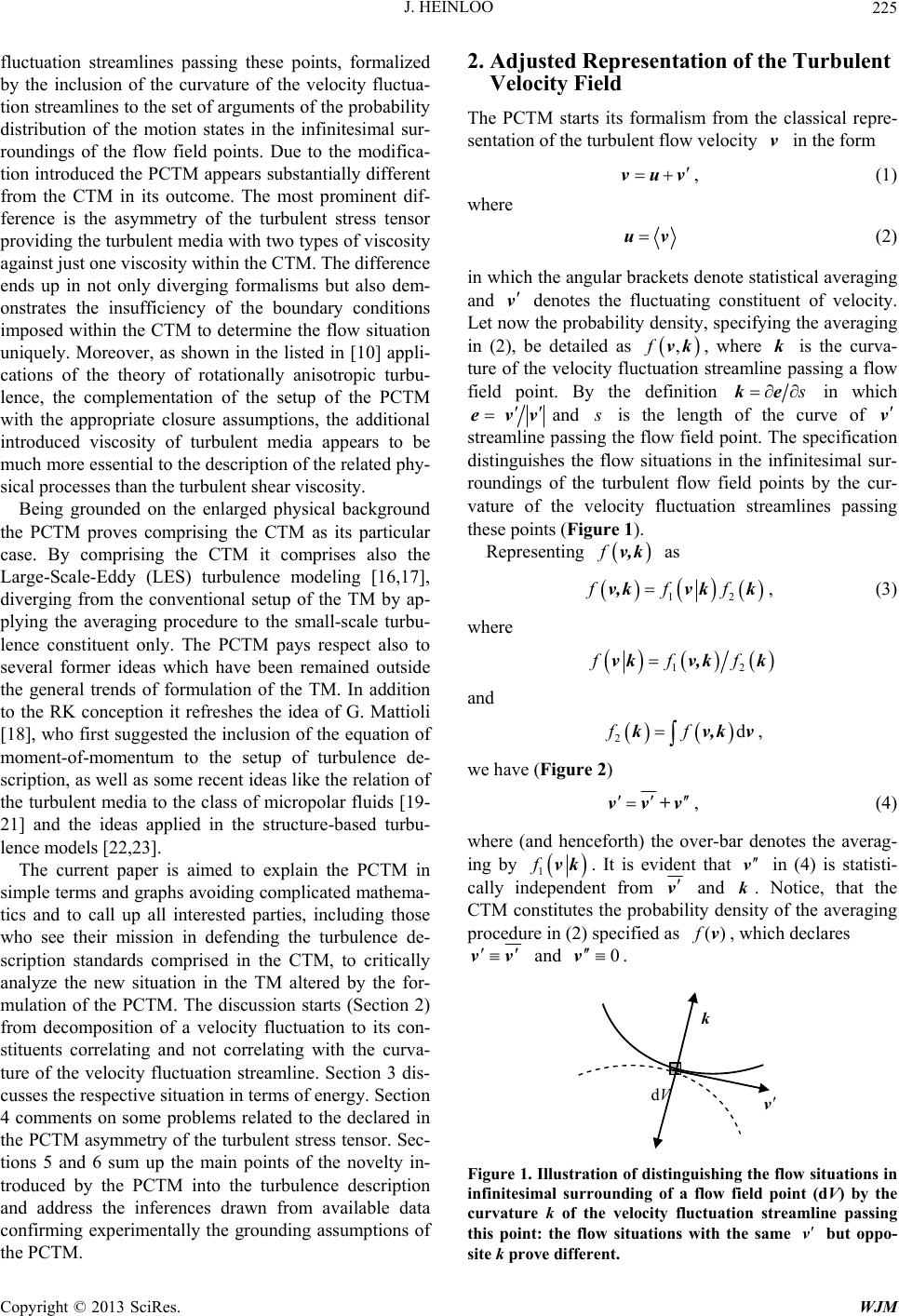

J. HEINLOO 225

fluctuation streamlines passing these points, formalized

by the inclusion of the curvature of the velocity fluctua-

tion streamlines to the set of arguments of the probability

distribution of the motion states in the infinitesimal sur-

roundings of the flow field points. Due to the modifica-

tion introduced the PCTM appears substantially different

from the CTM in its outcome. The most prominent dif-

ference is the asymmetry of the turbulent stress tensor

providing the tu rbulent media with two types of viscos ity

against just one viscosity within the CTM. The difference

ends up in not only diverging formalisms but also dem-

onstrates the insufficiency of the boundary conditions

imposed within the CTM to determine the flow situation

uniquely. Moreover, as shown in the listed in [10] appli-

cations of the theory of rotationally anisotropic turbu-

lence, the complementation of the setup of the PCTM

with the appropriate closure assumptions, the additional

introduced viscosity of turbulent media appears to be

much more essential to the description of the related ph y-

sical processes than the turbulent shear viscosity.

Being grounded on the enlarged physical background

the PCTM proves comprising the CTM as its particular

case. By comprising the CTM it comprises also the

Large-Scale-Eddy (LES) turbulence modeling [16,17],

diverging from the conventional setup of the TM by ap-

plying the averaging procedure to the small-scale turbu-

lence constituent only. The PCTM pays respect also to

several former ideas which have been remained outside

the general trends of formulation of the TM. In addition

to the RK conception it refreshes the idea of G. Mattioli

[18], who first suggested the inclusion of the equation of

moment-of-momentum to the setup of turbulence de-

scription, as well as some recent ideas like the relation of

the turbulent media to the class of micropolar fluids [19-

21] and the ideas applied in the structure-based turbu-

lence models [22,23].

The current paper is aimed to explain the PCTM in

simple terms and graphs avoiding complicated mathema-

tics and to call up all interested parties, including those

who see their mission in defending the turbulence de-

scription standards comprised in the CTM, to critically

analyze the new situation in the TM altered by the for-

mulation of the PCTM. The discussion starts (Section 2)

from decomposition of a velocity fluctuation to its con-

stituents correlating and not correlating with the curva-

ture of the velocity fluctuation streamline. Section 3 dis-

cusses the respective situation in terms of energy. Section

4 comments on some problems related to the declared in

the PCTM asymmetry of the turbu lent stress tensor. Sec-

tions 5 and 6 sum up the main points of the novelty in-

troduced by the PCTM into the turbulence description

and address the inferences drawn from available data

confirming experimentally the grounding assumptions of

the PCTM.

2. Adjusted Representation of the Turbulent

Velocity Field

The PCTM starts its formalism from the classical repre-

sentation of the turbulent flow velocity in the form





vuv, (1)

where

uv (2)

in which the an gular brackets denote statistical averag ing

and



v denotes the fluctuating constituent of velocity.

Let now the probability density, specifying the averaging

in (2), be detailed as





,fvk , where is the curva-

ture of the velocity fluctuation streamline passing a flow

field point. By the definition

 ke in which





vvand

is the length of the curve of



streamline passing the flow field point. The specification

distinguishes the flow situations in the infinitesimal sur-

roundings of the turbulent flow field points by the cur-

vature of the velocity fluctuation streamlines passing

these points (Fig ure 1).

Representing





fv,k as











fffv,kv kk, (3)

where







fffvkv,kk

and





2dff

kv,kv,

we have (Figure 2)





+vvv



, (4)

where (and henceforth) the over-bar denotes the averag-

ing by





fvk. It is evident that in (4) is statisti-

cally independent from





v and . Notice, that the

CTM constitutes the probability density of the averaging

procedure in (2) specified as

()

v, which declares





vv and 0







Figure 1. Illustration of distinguishing the flow situations in

infinitesimal surrounding of a flow field point (dV) by the

curvature k of the velocity fluctuation streamline passing

this point: the flow situations with the same



v but oppo-

site k prove different.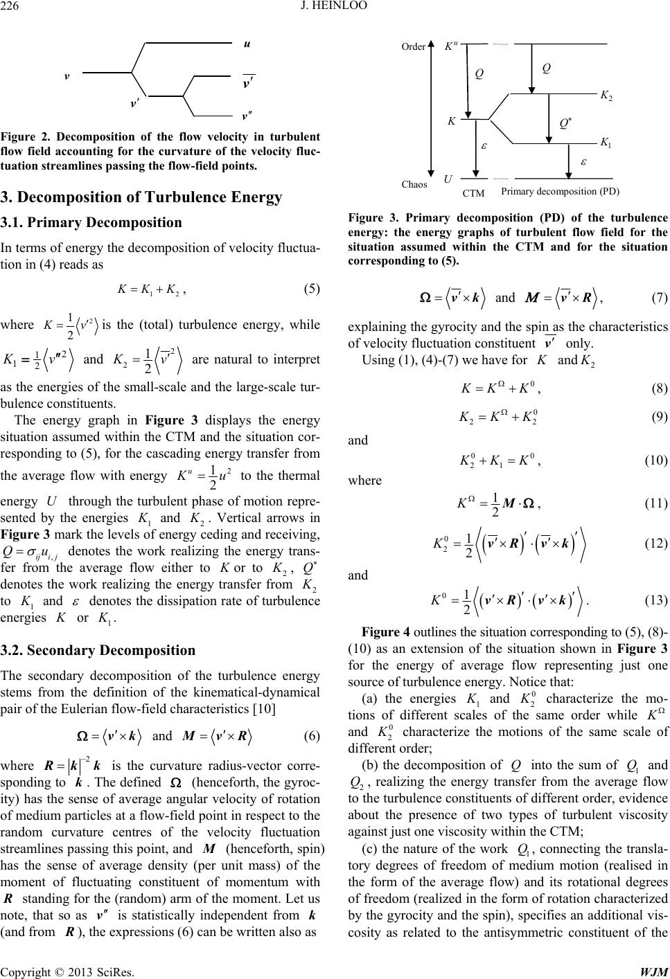

J. HEINLOO

226





Figure 2. Decomposition of the flow velocity in turbulent

flow field accounting for the curvature of the velocity fluc-

tuation streamlines passing the flow-field points.

3. Decomposition of Turbulence Energy

3.1. Primary Decomposition

In terms of energy the decomposition of velocity fluctu a-

tion in (4) reads as

KK, (5)

where 2

v

is the (total) turbulence energy, while

v

 and 2



 are natural to interpret

as the energies of the small-scale and the large-scale tur-

bulence constitu ents.

The energy graph in Figure 3 displays the energy

situation assumed within the CTM and the situation cor-

responding to (5), for the cascading energy transfer from

the average flow with energy 2

u to the thermal

energy through the turbulent phase of motion repre-

sented by the energies 1

and 2

. Vertical arrows in

Figure 3 mark the levels of energy ceding and receiving,

,iji j



 denotes the work realizing the energy trans-

fer from the average flow either to

or to 2

, Q



denotes the work realizing the energy transfer from 2

to 1

and



denotes the dissipation rate of turbulence

energies

or 1

3.2. Secondary Decomposition

The secondary decomposition of the turbulence energy

stems from the definition of the kinematical-dynamical

pair of the Euleri an fl o w -field characteristics [10]





vk and 



MvR (6)

where 2

Rkk is the curvature radius-vector corre-

sponding to . The defined



(henceforth, the gyroc-

ity) has the sense of average angular velocity of rotation

of medium particles at a flow-field point in respect to the

random curvature centres of the velocity fluctuation

streamlines passing this point, and (henceforth, spin)

has the sense of average density (per unit mass) of the

moment of fluctuating constituent of momentum w

Chaos

Order



Q

Primar y decomposition (PD)

CTM

Figure 3. Primary decomposition (PD) of the turbulence

energy: the energy graphs of turbulent flow field for the

situation assumed within the CTM and for the situation

corresponding to (5).





vk and 





, (7)

explaining the gyrocity and the spin as the characteristics

of velocity fluctuation constituent 

v only.

Using (1), (4)-(7) we have for

and2



, (8)



 (9)

and

21 0

KK, (10)

where 1

K



Μ, (11)



K



vR vk



(12)

and



K



vR vk



. (13)

Figure 4 outlines the situation corresponding to (5), (8)-

(10) as an extension of the situation shown in Figure 3

for the energy of average flow representing just one

source of turbulence energy. Notice that:

(a) the energies 1

and 0

characterize the mo-

tions of different scales of the same order while



and 0

characterize the motions of the same scale of

different order;

(b) the decomposition of into the sum of 1 and

2, realizing the energy transfer from the average flow

to the turbulence cons tituents of differen t orde r, eviden ce

about the presence of two types of turbulent viscosity

against just one viscosity within the CTM;

Q Q

tory degrees of freedom of medium motion (realised in

the form of the average flow) and its rotational degrees

of freedom (realized in the form of rotation characterized

by the gyrocity and the sp in), specifies an ad ditional vis-

cosity as related to the antisymmetric constituent of the

ith

standing for the (random) arm of the moment. Let us

note, that ss 

v is statistically independent fm k

(and f oro

rom a

), the expressions (6) can be written also as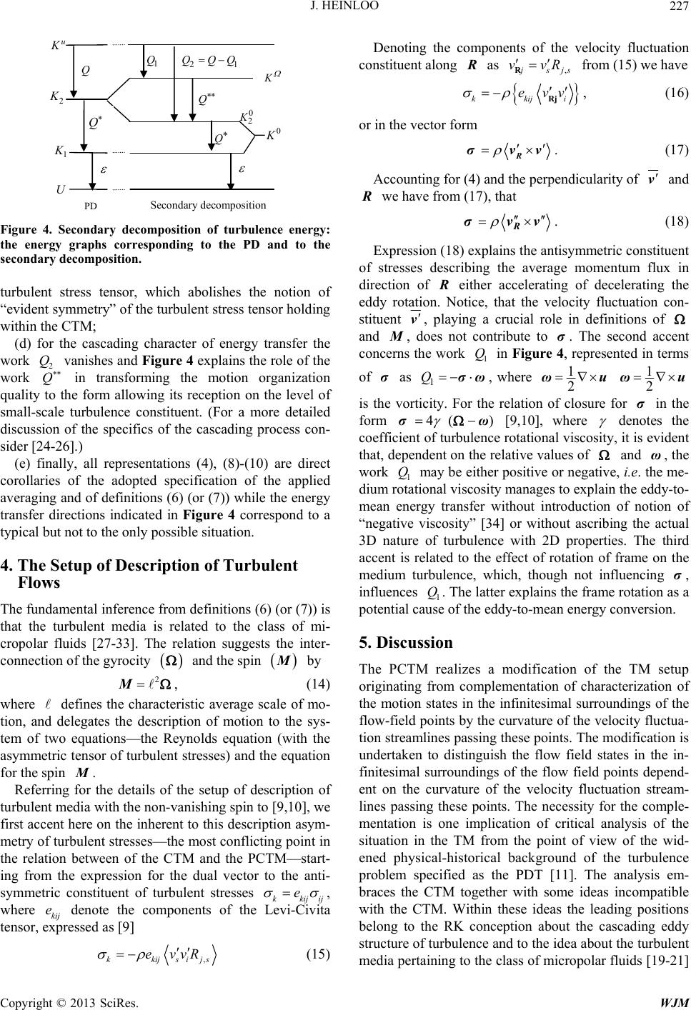

J. HEINLOO 227

Q



Q



QQQ



Q

Secondary decomposition

Figure 4. Secondary decomposition of turbulence energy:

the energy graphs corresponding to the PD and to the

secondary decomposition.

turbulent stress tensor, which abolishes the notion of

“evident symmetry” of the turb ulent stress tensor hold ing

within the CTM;

(d) for the cascading character of energy transfer the

work vanishes and Figure 4 explains the role of the

work in transforming the motion organization

quality to the form allowing its reception on the level of

small-scale turbulence constituent. (For a more detailed

discussion of the specifics of the cascading process con-

sider [24-26].)

Q

(e) finally, all representations (4), (8)-(10) are direct

corollaries of the adopted specification of the applied

averaging and of definitio ns (6) (or (7)) while the energy

transfer directions indicated in Figure 4 correspond to a

typical but not to the only possib le situation.

4. The Setup of Description of Turbulent

Flows

The fundamental inference from definitions (6) (or (7)) is

that the turbulent media is related to the class of mi-

cropolar fluids [27-33]. The relation suggests the inter-

connection of the gyrocity and the spin









M by

M, (14)

where defines the characteristic average scale of mo-

tion, and delegates the description of motion to the sys-

tem of two equations—the Reynolds equation (with the

asymmetric tensor of turbulent stresses) and the equation

for the spin .



Referring for the details of the setup of description of

turbulent medi a with th e non-v an ish ing sp in to [9 ,10 ], we

first accent here on the inherent to this description asym-

metry of turbulent stresses—th e most conflicting point in

the relation between of the CTM and the PCTM—start-

ing from the expression for the dual vector to the anti-

symmetric constituent of turbulent stresses kkij ij





where kij denote the components of the Levi-Civita

tensor, expressed as [9]

,kkijsij

evvR







Denoting the components of the velocity fluctuation

constituent along

as ,

sjs

vvR





R from (15) we have





kkij

evv





 Rj i

, (16)

or in the vector form







. (17)

Accounting for (4) and th e perpendicularity of



v and

we have from (17), that









vv. (18)

Expression (18) explains the an tisymmetric constitu ent

of stresses describing the average momentum flux in

direction of

either accelerating of decelerating the

eddy rotation. Notice, that the velocity fluctuation con-

stituent



v, playing a crucial role in definitions of



and , does not contribute to . The second accent

concerns the work in Figure 4, represen ted in terms

Mσ

of as

σ1



σω, where 1

ωu 1



ωu

is the vorticity. For the relation of closure for in the

form

σ4





()





[9,10], where



denotes the

coefficient of turbulence rotational viscosity, it is ev ident

that, dependent on the relative values of and ω, the

work 1 may be eith er positive or nega tive, i.e. the me-

dium rotational viscosity manages to explain the eddy-to-

mean energy transfer without introduction of notion of

“negative viscosity” [34] or without ascribing the actual

3D nature of turbulence with 2D properties. The third

accent is related to the effect of rotation of frame on the

medium turbulence, which, though not influencing ,

influences 1. The latter explains the frame rotation as a

potential cause of th e eddy-to-mean energy conversion.



5. Discussion

The PCTM realizes a modification of the TM setup

originating from complementation of characterization of

the motion states in the infinitesimal surroundings of the

flow-field points by the curvatur e of the velocity fluctua-

tion streamlines passing these points. Th e modification is

undertaken to distinguish the flow field states in the in-

finitesimal surroundings of the flow field points depend-

ent on the curvature of the velocity fluctuation stream-

lines passing these points. The necessity for the comple-

mentation is one implication of critical analysis of the

situation in the TM from the point of view of the wid-

ened physical-historical background of the turbulence

problem specified as the PDT [11]. The analysis em-

braces the CTM together with some ideas incompatible

with the CTM. Within these ideas the leading positions

belong to the RK conception about the cascading eddy

structure of turbulence and to the idea about the turbulent

media pertaining to the class of micropolar fluids [19-21]

(15)

J. HEINLOO

228

(as well as to the related to it earlier idea of G. Mattioli

[18], first suggesting the inclusion of the equation of

moment-of-momentum to the setup of description of tur-

bulent flows). The analysis displays the statement of the

CTM about the evident symmetry of the turbulent stress

tensor erring against the principles of continuum me-

chanics [15], relating the solution of the symmetry prop-

erties of the stress tensor to the context of specification

of the medium internal rotational degrees of freedom.

Within the shortcomings of th e CTM note also its inabil-

ity to propose ph ysically correct explanation to the eddy-

to-mean energy conversion, explained within the PCTM

as the act of turbulence rotational viscosity neglected

within the CTM. The CTM also does not distinguish the

turbulence properties in rotating and non-rotating frames

which by now is verified observationally.

Let us underline that the PCTM does not “discover”

the additional (rotational) viscosity of turbulence—this

type of turbulence viscosity has been foreseen and de-

scribed in a sufficiently complete form by the RK con-

ception—but merely removes the obstacle from the ex-

plicit inclusion of this fundamental property of turbu-

lence into the setup of the TM. Let us highlight also, that

applying all classical motion integrals—of momentum,

of moment-of-momentum and of energy—the PCTM

formulates the turbulence description in mechanically

closed form and as such completes the formulation of the

TM.

We conclude the comments on the PCTM referring to

the paper [35], which utilized the data available within

the Global Drifter Program to estimate the gyrocity and

the spin immediately from observations. The estimated

gyrocity and spin provide the grounding declaration of

the PCTM about the non-vanishing gyrocity and spin of

the turbulent flow with the sense of experimental fact.

Finally, the PDT [11] postulates the conditions of for-

mation of probability distribution properties of momen-

tary states of motion determined as the state of motion

fixed in terms of the TM. These conditions are specified

within the CTM and within the PCTM differently. The

commented role of the TM is emphasized here to stress

the scientific merit of the TM wider than a particular

turbulence description in average terms.

6. Conclusion

The PCTM mandates a critical analysis of the results

following from the CTM. It also mandates the planning

of new tasks and research projects from the position of

the PCTM. The latter mandate is addressed to the initia-

tors of new projects rather than hug e number of scien tists

participating in turbulence-related applied projects and

following firmly established standards. This mandate is

also addressed to the people educating new generation of

specialists in the field of flu id mechanics.

REFERENCES

[1] J. Boussinesq, “Théorie de l’Ecoulement Tourbillant,”

Mém. prés. Acad. Sci., Vol. XXIII, 1877, p. 46.

[2] O. Reynolds, “On the Dynamical Theory of Incompressi-

ble Viscous Fluids and Determination of the Criterion,”

Philosophical Transactions of the Royal Society, Vol. 186,

1884, pp. 123-161.

[3] L. Prandtl, “Über die Ausgebildete Turbulentz,” ZAMM,

Vol. 5, 1925, pp. 136-139.

[4] G. I. Taylor, “The Transport of Vorticity and Heat through

Fluids in Turbulent Motion,” Proceedings of the Royal

Society A, Vol. 135, 1932, pp. 685-705.

[5] D. C. Wilcox, “Turbulence Modeling for CFD,” 2nd Edi-

tion, DCW Industries, Anaheim, 1998.

[6] B. E. Launder and B. I. Sharma, “Application of the En-

ergy Dissipation Model of Turbulence to the Calculation

of Flow near a Spinning Disc,” Letters in Heat and Mass

Transfer, Vol. 1, No. 2, 1974, pp. 131-138.

[7] L. F. Richardson, “Weather Prediction by Numerical Pro-

cess,” Cambridge University Press, Cambridge, 1922.

[8] A. N. Kolmogorov, “The Local Structure of Turbulence

in Incompressible Viscous Fluids for Very Large Rey-

nolds Numbers,” Doklady Akademii Nauk SSSR, Vol. 30,

1941, pp. 376-387 (in Russian).

[9] J. Heinloo, “Formulation of Turbulence Mechanics,”

Physical Review E, Vol. 69, 2004, Article ID: 056317.

doi:10.1103/PhysRevE.69.056317

[10] J. Heinloo, “Postclassical Turbulence Mechanics,” Jour-

nal of Modern Physics, Vol. 4, No. 4, 2013, pp. 505-516.

doi:10.4236/jmp.2013.44072

[11] J. Heinloo, “Physical Doctrine of Turbulence,” Interna-

tional Journal of Research and Reviews in Applied Sci-

ences, Vol. 12, No. 2, 2012, pp. 214-221.

[12] J. Heinloo, “On Description of Stochastic Systems,”

Proceedings of the Estonian Academy of Sciences, Phys-

ics and Mathematics, Vol. 53, No. 3, 2004, pp. 186-200.

[13] J. Heinloo, “A Setup of Systemic Description of Fluids

Motion,” Proceedings of the Estonian Academy of Sci-

ences, Vol. 58, No. 3, 2009, pp. 184-189.

doi:10.3176/proc.2009.3.05

[14] A. Ishiara, “Statistical Physics,” Academic Press, New

York, London, 1971.

[15] L. I. Sedov, “A Course in Continuum Mechanics,” Klu-

wer, 1987.

[16] M. Lesieur, O. Métais and P Comte, “Large-Eddy Simu-

lations of Turbulence,” Cambridge University Press, Cam-

bridge, 2005. doi:10.1017/CBO9780511755507

[17] P. Sagaut, “Large Eddy Simulation for Incompressible

Flows,” Springer, Berlin, Heidelberg, 2006.

[18] G. D. Mattioli, “Teoria Dinamica dei Regimi Fluidi Tur-

bolenti,” Padova, 1937.

[19] A. C. Eringen, “Micromorphic Description of Turbulent

Channel Flow,” Journal of Mathematical Analysis and

Applications, Vol. 39, No. 1, 1972, pp. 253-266.

doi:10.1016/0022-247X(72)90239-9

J. HEINLOO

229

[20] A. C. Eringen and T. S. Chang, “Micropolar Description

of Hydrodynamic Turbulence,” Advances in Materials

Science and Engineering, Vol. 5, No. 1, 1970, pp.1-8.

[21] J. Peddieson, “An Application of the Micropolar Fluid

Model to Calculation of Turbulent Shear Flow,” Interna-

tional Journal of Engineering Science, Vol. 10, No. 1,

1972, pp. 23-32. doi:10.1016/0020-7225(72)90072-9

[22] W. C. Reynolds, C. A. Langer and S. C. Kassinos, “Struc-

ture and Scales in Turbulence Modeling,” Physics of Flu-

ids, Vol. 14, No. 7, 2002, pp. 2485-2492.

doi.10.1063/1.1473784

[23] S. C. Kassinos and W. C. Reynolds, “Developments in

Structure-Based Turbulence Modeling,” In: M. D. Salas, J.

N. Hefner and L. Sakell, Eds., Modeling Complex Turbu-

lent Flows, Kluwer, 1999, pp. 69-87.

[24] J. Heinloo, “The Structure of Average Turbulent Flow

Field,” Central European Journal of Physics, Vol. 8, No.

1, 2010, pp. 17-24. doi:10.2478/s11534-009-0015-y

[25] J. Heinloo, “Setup of Turbulence Mechanics Accounting

for a Preferred Orientation of Eddy Rotation,” Concepts

of Physics, Vol. 5, No. 2, 2008, pp. 205-219.

doi:10.2478/v10005-007-0033-8

[26] J. Heinloo, “A Generalized Setup of the Turbulence De-

scription,” Advanced Studies in Theoretical Physics, Vol.

5, No. 10, 2011, pp. 477-483.

[27] T. Ariman, M. A. Turk and D. O. Silvester, “Microcon-

tinuum Fluid Mechanics A Review,” International Jour-

nal of Engineering Science, Vol. 11, No. 8, 1973, pp.

905-930. doi:10.1016/0020-7225(73)90038-4

[28] D. W. Condiff and J. S. Dahler, “Fluid Mechanical As-

pects of Antisymmetric Stress,” Physics of Fluids, Vol. 7,

1964, pp. 842-854. doi.org/10.1063/1.1711295

[29] J. S. Dahler, “Transport Phenomena in a Fluid Composed

of Diatomic Molecules,” Journal of Chemical Physics,

Vol. 30, 1959, pp. 1447-1475. doi.org/10.1063/1.1730220

[30] J. S. Dahler and L. F. Scriven, “Angular Momentum of

Continua,” Nature, Vol. 192, No. 4797, 1961, pp. 36-37.

doi:10.1038/192036a0

[31] J. S. Dahler and L. F. Scriven, “Theory of Structured

Continua: General Consideration of Angular Momentum

and Polarization,” Proceedings of the Royal Society, Vol.

A275, 1963, pp. 504-527.

[32] A. C. Eringen, “Theory of Micropolar Fluids,” Mathe-

matics and Mechanics, Vol. 16, No. 1, 1966, pp. 1-18.

[33] A. C. Eringen, “Mechanics of Micropolar Continua,” In:

E. Kröner, Ed., Mechanics of Generalized Continua,

Springer-Verlag, Berlin, 1968, pp. 18-35.

[34] P. Starr, “Physics of Negative Viscosity Phenomena,”

McGrav-Hill, New York, 1968.

[35] J. Heinloo and A. Toompuu, “Gyration Effect of the

Large-Scale Turbulence in the Upper Ocean,” Environ-

mental Fluid Mechanics, Vol. 12, No. 5, 2012, pp. 429-

438. doi:10.1007/s10652-012-9247-2