Fully and Partly Divergence and Rotation Free Interpolation of Magnetic Fields

doi:10.4236/jemaa.2013.57044

Paper Menu >>

Journal Menu >>

Journal of Electromagnetic Analysis and Applications, 2013, 5, 281-287

http://dx.doi.org/10.4236/jemaa.2013.57044 Published Online July 2013 (http://www.scirp.org/journal/jemaa)

281

Fully and Partly Divergence and Rotation Free

Interpolation of Magnetic Fields

Victor-Otto de Haan

BonPhysics Research and Investigations B.V., Laan van Heemstede 38, 3297 AJ Puttershoek, The Netherlands.

Email: [email protected]

Received May 31st, 2013; revised July 1st, 2013; accepted July 9th, 2013

which permits unrestricted use, distribution, and reproduction in any medium, provided the original work is properly cited.

ABSTRACT

A new interpolation method for rotation and divergence free fields is presented. It is based on a suitable choice of a

tricubic interpolation scheme and reaches an accuracy of third order in grid size (Δx). With the interpolation method it is

possible to increase the accuracy with a factor of grid size/distance with respect to the trilinear interpolation method

using exactly the same data points. Simulations for several distances of dipoles (r) to the interpolation area show that

the maximum relative deviation is approximately 3(Δx/r)3 ppm.

Keywords: Magnetic Fields; Interpolation; Magnetic Field Measurement

1. Introduction

For many applications it is needed that a vector field is

accurately known with sufficient spatial resolution. For

instance for the calculation of neutron spin precession [1],

in magnetic resonance imaging [2] or in space [3]. In

case these magnetic fields can be calculated, it is possible

that these calculations are very time consuming and it

might be impossible to do these calculations with the

required spatial resolution. In case these magnetic fields

have to be measured, it is also possible (and even likely)

that these measurements are very time consuming and

the required spatial resolution can not be obtained. In

these cases one must resort to interpolation methods. It is

important to have an interpolation method that is accu-

rately enough, even when the grid size of the calculated

or measured data is large with respect to the required

resolution. This calls for higher order interpolation

schemes. The use of a divergence and rotation free in-

terpolation can be advantageous in two respects. First, by

using these properties of the field it is possible to in-

crease the accuracy of the interpolation. Second, in some

cases if the interpolated field is not rotation and diver-

gence free, this leads to erroneous results which have no

physical meaning. This is the case in for instance mag-

neto-hydrodynamics [4]. An important example of a ro-

tation and divergence free vector field is the magnetic

field in a conduction current free region in a homogene-

ous material. The magnetic field is always divergence

free and when there are no conduction currents, the field

is also rotation free. In literature various methods exist

based on a trilinear [5], triquadratic, or even tricubic [6]

interpolation schemes. The disadvantages of these meth-

ods are either their limited accuracy (trilinear and tri-

quadratic) or the large number of grid points needed

(triquadratic and tricubic). Further, in general, these in-

terpolation methods result in a field inside the grid that

has a finite divergence and rotation, possibly resulting in

unphysical results. Here, a method is presented that gives

a rotation and divergence free interpolation of a vector

field inside a 3D-rectangular grid, with an accuracy that

is third order in grid size.

2. Method

Lets consider a rectangular box of homogeneous material

(with linear constitutive equations) with sides Δx, Δy and

Δz (see also Figure 1). The Maxwell equations require

that the magnetic induction is always divergence free. In

case of the quasi-static limit and without conduction cur-

rents the magnetic induction should also be rotation free.

As the material is homogeneous and linear, these condi-

tions also hold for the magnetic field,

A rotation free field can always be described as the

gradient of a scalar quantity, so let us define a scalar field,

G so that

G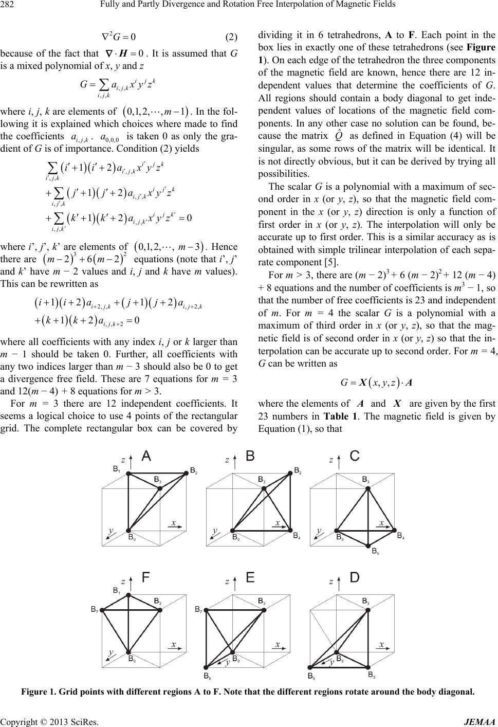

(1)

then

Fully and Partly Divergence and Rotation Free Interpolation of Magnetic Fields

282

20G (2)

because of the fact that 0

. It is assumed that G

is a mixed polynomial of x, y and z

ijk

Gaxyz

where i, j, k are elements of





0,1,2,,1m. In the fol-

lowing it is explained which choices where made to find

the coefficients ,,ijk. 0,0,0 is taken 0 as only the gra-

dient of G is of importance. Condition (2) yields

a a

 

ijk

iiaxyz

jjaxyz

kkaxyz













 



0



where i’, j’, k’ are elements of . Hence

there are equations (note that

i’, j’

and k’ have m − 2 values and i, j and k have m values).

This can be rewritten as



0,1,2,, 3m





26 2mm 





 



2, ,,2,

,, 2

121 2

12 0

ijk ijk

ijk

iiaj ja

kka





 



where all coefficients with any index i, j or k larger than

m − 1 should be taken 0. Further, all coefficients with

any two indices larger than m − 3 should also be 0 to get

a divergence free field. These are 7 equations for m = 3

and 12(m − 4) + 8 equations for m > 3.

For m = 3 there are 12 independent coefficients. It

seems a logical choice to use 4 points of the rectangular

grid. The complete rectangular box can be covered by

dividing it in 6 tetrahedrons, A to F. Each point in the

box lies in exactly one of these tetrahedrons (see Figure

1). On each edge of the tetrahedron the three components

of the magnetic field are known, hence there are 12 in-

dependent values that determine the coefficients of G.

All regions should contain a body diagonal to get inde-

pendent values of locations of the magnetic field com-

ponents. In any other case no solution can be found, be-

cause the matrix as defined in Equation (4) will be

singular, as some rows of the matrix will be identical. It

is not directly obvious, but it can be derived by trying all

possibilities.

The scalar G is a polynomial with a maximum of sec-

ond order in x (or y, z), so that the magnetic field com-

ponent in the x (or y, z) direction is only a function of

first order in x (or y, z). The interpolation will only be

accurate up to first order. This is a similar accuracy as is

obtained with simple trilinear interpolation of each sepa-

rate component [5].

For m > 3, there are (m − 2)3 + 6 (m − 2)2 + 12 (m − 4)

+ 8 equations and the number of coefficients is m3 − 1, so

that the number of free coefficients is 23 and independent

of m. For m = 4 the scalar G is a polynomial with a

maximum of third order in x (or y, z), so that the mag-

netic field is of second order in x (or y, z) so that the in-

terpolation can be accurate up to second order. For m = 4,

G can be written as





,,Gxyz





where the elements of

and

are given by the first

23 numbers in Table 1. The magnetic field is given by

Equation (1), so that

Figure 1. Grid points with different regions A to F. Note that the different regions rotate around the body diagonal.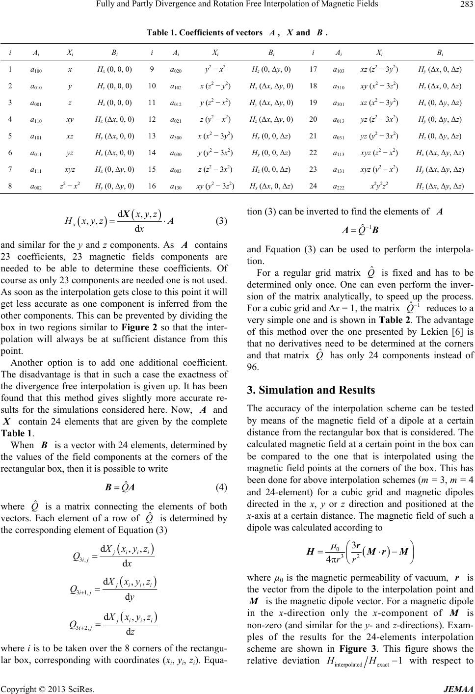

Fully and Partly Divergence and Rotation Free Interpolation of Magnetic Fields 283

Table 1. Coefficients of vectors ,

and . B

i Ai X

i B

i i Ai X

i B

i i Ai X

i B

1 a100 x Hx (0, 0, 0) 9 a020 y2 − x2 Hz (0, Δy, 0) 17 a103 xz (z2 − 3y2) Hy (Δx, 0, Δz)

2 a010 y Hy (0, 0, 0) 10 a102 x (z2 − y2) Hx (Δx, Δy, 0) 18 a310 xy (x2 − 3z2) Hz (Δx, 0, Δz)

3 a001 z Hz (0, 0, 0) 11 a012 y (z2 − x2) Hy (Δx, Δy, 0) 19 a301 xz (x2 − 3y2) Hx (0, Δy, Δz)

4 a110 xy Hx (Δx, 0, 0) 12 a021 z (y2 − x2) Hz (Δx, Δy, 0) 20 a013 yz (z2 − 3x2) Hy (0, Δy, Δz)

5 a101 xz Hy (Δx, 0, 0) 13 a300 x (x2 − 3y2) Hx (0, 0, Δz) 21 a031 yz (y2 − 3x2) Hz (0, Δy, Δz)

6 a011 yz Hz (Δx, 0, 0) 14 a030 y (y2 − 3x2) Hy (0, 0, Δz) 22 a113 xyz (z2 − x2) Hx (Δx, Δy, Δz)

7 a111 xyz Hx (0, Δy, 0) 15 a003 z (z2 − 3x2) Hz (0, 0, Δz) 23 a131 xyz (y2 − x2) Hy (Δx, Δy, Δz)

8 a002 z2 − x2 Hy (0, Δy, 0) 16 a130 xy (y2 − 3z2)Hx (Δx, 0, Δz) 24 a222 x2y2z2 Hz (Δx, Δy, Δz)



d,,

,, d

xyz

Hxyz



XA (3)

and similar for the y and z components. As

contains

23 coefficients, 23 magnetic fields components are

needed to be able to determine these coefficients. Of

course as only 23 components are needed one is not used.

As soon as the interpolation gets close to this point it will

get less accurate as one component is inferred from the

other components. This can be prevented by dividing the

box in two regions similar to Figure 2 so that the inter-

polation will always be at sufficient distance from this

point.

Another option is to add one additional coefficient.

The disadvantage is that in such a case the exactness of

the divergence free interpolation is given up. It has been

found that this method gives slightly more accurate re-

sults for the simulations considered here. Now,

and

contain 24 elements that are given by the complete

Table 1.

When is a vector with 24 elements, determined by

the values of the field components at the corners of the

rectangular box, then it is possible to write

Q

BA (4)

where is a matrix connecting the elements of both

vectors. Each element of a row of is determined by

the corresponding element of Equation (3)

Qˆ





d,,

iii

xyz







31,

d,,

iii

xyz







32,

d,,

iii

xyz



where i is to be taken over the 8 corners of the rectangu-

lar box, corresponding with coordinates (xi, yi, zi). Equa-

tion (3) can be inverted to find the elements of

Q



and Equation (3) can be used to perform the interpola-

tion.

For a regular grid matrix is fixed and has to be

determined only once. One can even perform the inver-

sion of the matrix analytically, to speed up the process.

For a cubic grid and Δx = 1, the matrix reduces to a

very simple one and is shown in Table 2. The advantage

of this method over the one presented by Lekien [6] is

that no derivatives need to be determined at the corners

and that matrix has only 24 components instead of

96.

Q

3. Simulation and Results

The accuracy of the interpolation scheme can be tested

by means of the magnetic field of a dipole at a certain

distance from the rectangular box that is considered. The

calculated magnetic field at a certain point in the box can

be compared to the one that is interpolated using the

magnetic field points at the corners of the box. This has

been done for above interpolation schemes (m = 3, m = 4

and 24-element) for a cubic grid and magnetic dipoles

directed in the x, y or z direction and positioned at the

x-axis at a certain distance. The magnetic field of such a

dipole was calculated according to



4rr











r

MrM

where µ0 is the magnetic permeability of vacuum, is

the vector from the dipole to the interpolation point and

is the magnetic dipole vector. For a magnetic dipole

in the x-direction only the x-component of is

non-zero (and similar for the y- and z-directions). Exam-

ples of the results for the 24-elements interpolation

scheme are shown in Figure 3. This figure shows the

relative deviation

interpolatedexact 1HH with respect to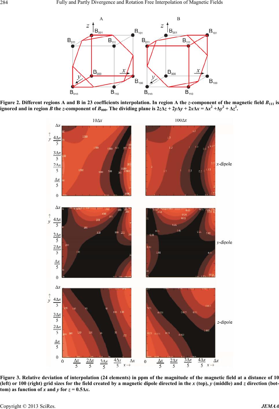

Fully and Partly Divergence and Rotation Free Interpolation of Magnetic Fields

284

A B

Figure 2. Different regions A and B in 23 coefficients interpolation. In region A the z-component of the magnetic field B111 is

ignored and in region B the z-component of B000. The dividing plane is 2zΔz + 2yΔy + 2xΔx = Δx2 +Δy2 + Δz2.

Figure 3. Relative deviation of interpolation (24 elements) in ppm of the magnitude of the magnetic field at a distance of 10

(left) or 100 (right) grid sizes for the field created by a magnetic dipole directed in the x (top), y (middle) and z direction (bot-

tom) as function of x and y for z = 0.5Δx.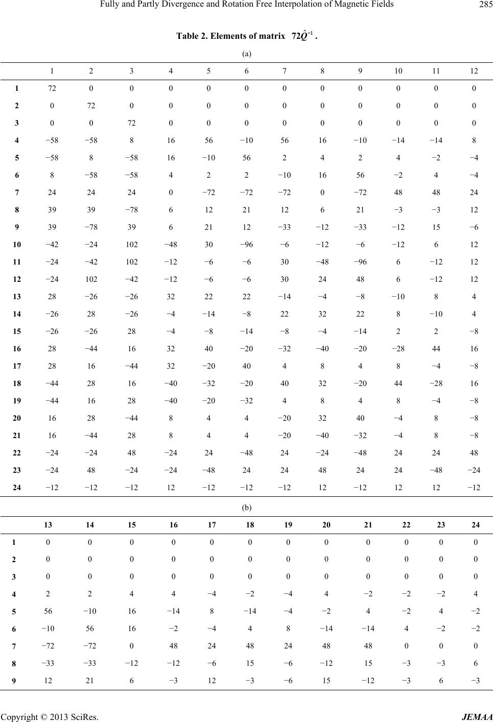

Fully and Partly Divergence and Rotation Free Interpolation of Magnetic Fields 285

Table 2. Elements of matrix ˆ

72Q

-1

(a)

1 2 3 4 5 6 7 8 9 10 11 12

1 72 0 0 0 0 0 0 0 0 0 0 0

2 0 72 0 0 0 0 0 0 0 0 0 0

3 0 0 72 0 0 0 0 0 0 0 0 0

4 −58 −58 8 16 56 −10 56 16 −10 −14 −14 8

5 −58 8 −58 16 −10 56 2 4 2 4 −2 −4

6 8 −58 −58 4 2 2 −10 16 56 −2 4 −4

7 24 24 24 0 −72 −72 −72 0 −72 48 48 24

8 39 39 −78 6 12 21 12 6 21 −3 −3 12

9 39 −78 39 6 21 12 −33 −12 −33 −12 15 −6

10 −42 −24 102 −48 30 −96 −6 −12 −6 −12 6 12

11 −24 −42 102 −12 −6 −6 30 −48 −96 6 −12 12

12 −24 102 −42 −12 −6 −6 30 24 48 6 −12 12

13 28 −26 −26 32 22 22 −14 −4 −8 −10 8 4

14 −26 28 −26 −4 −14 −8 22 32 22 8 −10 4

15 −26 −26 28 −4 −8 −14 −8 −4 −14 2 2 −8

16 28 −44 16 32 40 −20 −32 −40 −20 −28 44 16

17 28 16 −44 32 −20 40 4 8 4 8 −4 −8

18 −44 28 16 −40 −32 −20 40 32 −20 44 −28 16

19 −44 16 28 −40 −20 −32 4 8 4 8 −4 −8

20 16 28 −44 8 4 4 −20 32 40 −4 8 −8

21 16 −44 28 8 4 4 −20 −40 −32 −4 8 −8

22 −24 −24 48 −24 24 −48 24 −24 −48

24 24 48

23 −24 48 −24 −24 −48 24 24 48 24 24 −48 −24

24 −12 −12 −12 12 −12 −12 −12 12 −12 12 12 −12

(b)

13 14 15 16 17 18 19 20 21 22 23 24

1 0 0 0 0 0 0 0 0 0 0 0 0

2 0 0 0 0 0 0 0 0 0 0 0 0

3 0 0 0 0 0 0 0 0 0 0 0 0

4 2 2 4 4 −4 −2 −4 4 −2 −2 −2 4

5 56 −10 16 −14 8 −14 −4 −2 4 −2 4 −2

6 −10 56 16 −2 −4 4 8 −14 −14 4 −2 −2

7 −72 −72 0 48 24 48 24 48 48 0 0 0

8 −33 −33 −12 −12 −6 15 −6 −12 15 −3 −3 6

9 12 21 6 −3 12 −3 −6 15 −12 −3 6 −3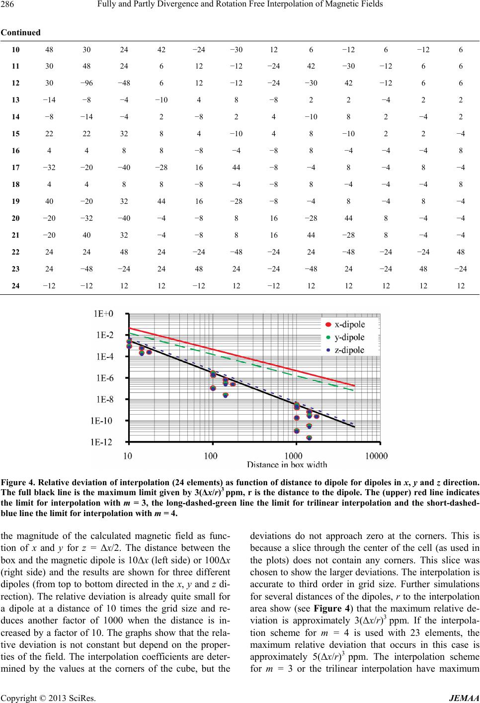

Fully and Partly Divergence and Rotation Free Interpolation of Magnetic Fields

286

Continued

10 48 30 24 42 −24 −30 12 6 −12 6 −12 6

11 30 48 24 6 12 −12 −24 42 −30 −12 6 6

12 30 −96 −48 6 12 −12 −24 −30 42 −12 6 6

13 −14 −8 −4 −10 4 8 −8 2 2 −4 2 2

14 −8 −14 −4 2 −8 2 4 −10 8 2 −4 2

15 22 22 32 8 4 −10 4 8 −10 2 2 −4

16 4 4 8 8 −8 −4 −8 8 −4 −4 −4 8

17 −32 −20 −40 −28 16 44 −8 −4 8 −4 8 −4

18 4 4 8 8 −8 −4 −8 8 −4 −4 −4 8

19 40 −20 32 44 16 −28 −8 −4 8 −4 8 −4

20 −20 −32 −40 −4 −8 8 16 −28 44 8 −4 −4

21 −20 40 32 −4 −8 8 16 44 −28 8 −4 −4

22 24 24 48 24 −24 −48 −24 24 −48 −24 −24 48

23 24 −48 −24 24 48 24 −24 −48 24 −24 48 −24

24 −12 −12 12 12 −12 12 −12 12 12 12 12 12

Figure 4. Relative deviation of interpolation (24 elements) as function of distance to dipole for dipoles in x, y and z direction.

The full black line is the maximum limit given by 3(Δx/r)3 ppm, r is the distance to the dipole. The (upper) red line indicates

the limit for interpolation with m = 3, the long-dashed-green line the limit for trilinear interpolation and the short-dashed-

blue line the limit for interpolation with m = 4.

the magnitude of the calculated magnetic field as func-

tion of x and y for z = Δx/2. The distance between the

box and the magnetic dipole is 10Δx (left side) or 100Δx

(right side) and the results are shown for three different

dipoles (from top to bottom directed in the x, y and z di-

rection). The relative deviation is already quite small for

a dipole at a distance of 10 times the grid size and re-

duces another factor of 1000 when the distance is in-

creased by a factor of 10. The graphs show that the rela-

tive deviation is not constant but depend on the proper-

ties of the field. The interpolation coefficients are deter-

mined by the values at the corners of the cube, but the

deviations do not approach zero at the corners. This is

because a slice through the center of the cell (as used in

the plots) does not contain any corners. This slice was

chosen to show the larger deviations. The interpolation is

accurate to third order in grid size. Further simulations

for several distances of the dipoles, r to the interpolation

area show (see Figure 4) that the maximum relative de-

viation is approximately 3(Δx/r)3 ppm. If the interpola-

tion scheme for m = 4 is used with 23 elements, the

maximum relative deviation that occurs in this case is

approximately 5(Δx/r)3 ppm. The interpolation scheme

for m = 3 or the trilinear interpolation have maximum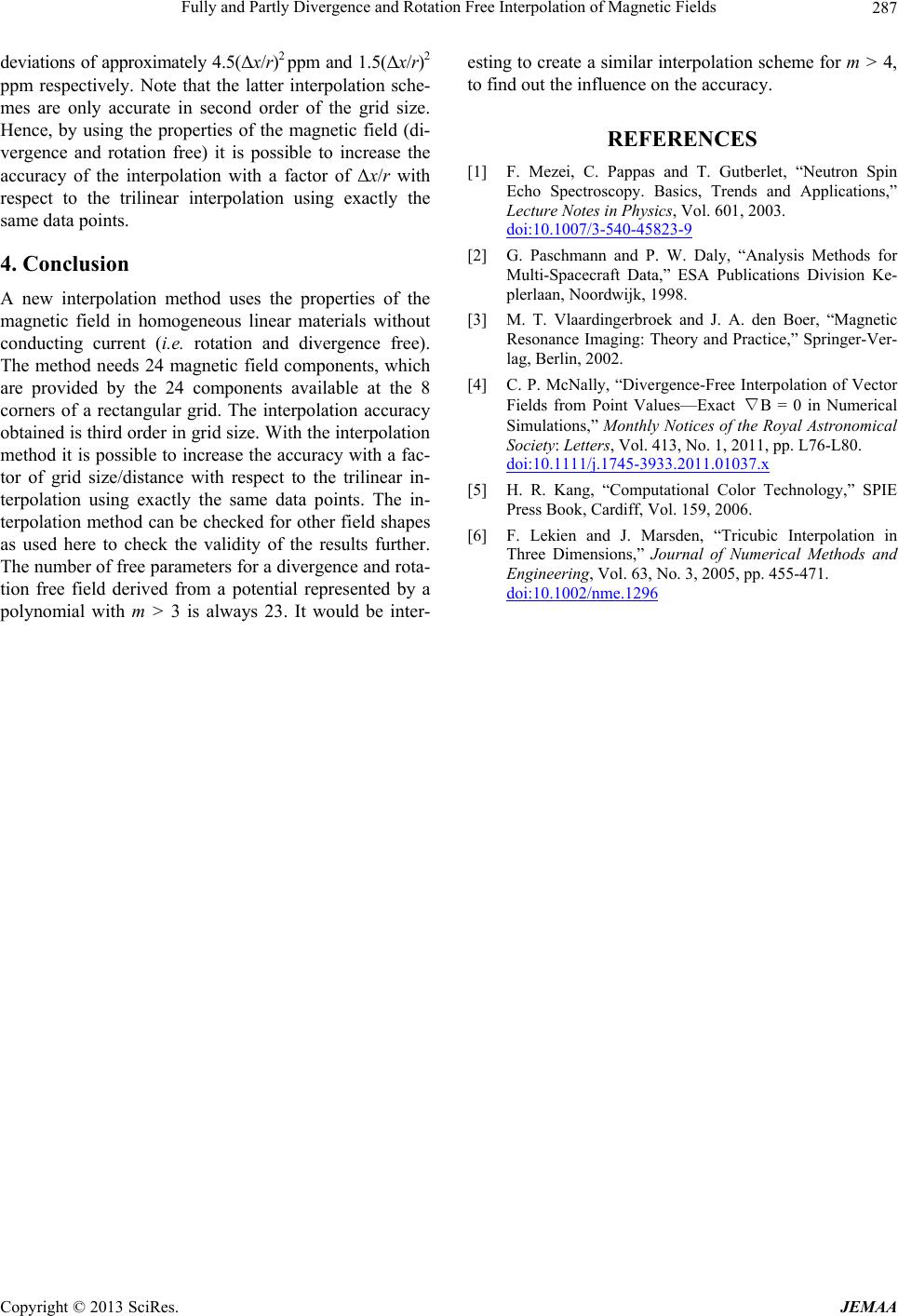

Fully and Partly Divergence and Rotation Free Interpolation of Magnetic Fields 287

deviations of approximately 4.5(Δx/r)2 ppm and 1.5(Δx/r)2

ppm respectively. Note that the latter interpolation sche-

mes are only accurate in second order of the grid size.

Hence, by using the properties of the magnetic field (di-

vergence and rotation free) it is possible to increase the

accuracy of the interpolation with a factor of Δx/r with

respect to the trilinear interpolation using exactly the

same data points.

4. Conclusion

A new interpolation method uses the properties of the

magnetic field in homogeneous linear materials without

conducting current (i.e. rotation and divergence free).

The method needs 24 magnetic field components, which

are provided by the 24 components available at the 8

corners of a rectangular grid. The interpolation accuracy

obtained is third order in grid size. With the interpolation

method it is possible to increase the accuracy with a fac-

tor of grid size/distance with respect to the trilinear in-

terpolation using exactly the same data points. The in-

terpolation method can be checked for other field shapes

as used here to check the validity of the results further.

The number of free parameters for a divergence and rota-

tion free field derived from a potential represented by a

polynomial with m > 3 is always 23. It would be inter-

esting to create a similar interpolation scheme for m > 4,

to find out the influence on the accuracy.

REFERENCES

[1] F. Mezei, C. Pappas and T. Gutberlet, “Neutron Spin

Echo Spectroscopy. Basics, Trends and Applications,”

Lecture Notes in Physics, Vol. 601, 2003.

doi:10.1007/3-540-45823-9

[2] G. Paschmann and P. W. Daly, “Analysis Methods for

Multi-Spacecraft Data,” ESA Publications Division Ke-

plerlaan, Noordwijk, 1998.

[3] M. T. Vlaardingerbroek and J. A. den Boer, “Magnetic

Resonance Imaging: Theory and Practice,” Springer-Ver-

lag, Berlin, 2002.

[4] C. P. McNally, “Divergence-Free Interpolation of Vector

Fields from Point Values—Exact ∇B = 0 in Numerical

Simulations,” Monthly Notices of the Royal Astronomical

Society: Letters, Vol. 413, No. 1, 2011, pp. L76-L80.

doi:10.1111/j.1745-3933.2011.01037.x

[5] H. R. Kang, “Computational Color Technology,” SPIE

Press Book, Cardiff, Vol. 159, 2006.

[6] F. Lekien and J. Marsden, “Tricubic Interpolation in

Three Dimensions,” Journal of Numerical Methods and

Engineering, Vol. 63, No. 3, 2005, pp. 455-471.

doi:10.1002/nme.1296