Atmospheric Dispersion and Deposition of Radionuclides (<sup>137</sup>Cs and <sup>131</sup>I) Released from the Fukushima Dai-ichi Nuclear Power Plant

doi:10.4236/cweee.2013.22B011

Paper Menu >>

Journal Menu >>

Computational Water, Energy, and Environmental Engineering, 2013, 2, 61-68

doi:10.4236/cweee.2013.22B011 Published Online April 2013 (http://www.scirp.org/journal/cweee)

Atmospheric Dispersion and Deposition of Radionuclides

(137Cs and 131I) Released from the Fukushima Dai-ichi

Nuclear Power Plant

Soon-Ung Park, Anna Choe, Moon-Soo Park

Center for Atmospheric and Environmental Modeling, Seoul, Korea

Email: [email protected]r

Received 2013

ABSTRACT

The Lagrangian Particle Dispersion Model (LPDM) in the 594 km × 594 km model domain with the horizontal grid

scale of 3 km × 3 km centered at a po wer plant and the Eulerian Transport Model (ETM) modified from the Asian Dust

Aerosol Model 2 (ADAM2) in the domain of 70° LAT × 140° LON with the horizontal grid scale of 27 km × 27 km

have been developed. These models have been implemented to simulate the concentration and deposition of radionuc-

lides (137Cs and 131I) released from the accide nt of the Fukushi ma Dai-ic hi nuclear p ower plant. I t is found that both

models are able to simulate quite reasonably the observed concentrations of 137Cs and 131I near the power plant.

However, the LPDM model is more useful for the estimation of concentration near the power plant site in details whe-

reas the ETM model is good for the long-range transport processes of the radionuclide plume. T he estimated maximum

mean surface concentration, column integrated mean concentration and the total deposition (wet+dry) by LPDM for the

period from 12 March to 30 April 2011 are, respectively found to be 2.975 × 102 Bq m-3, 3.7 × 107 Bq m-2, and 1.78 ×

1014 Bq m-2 for 137Cs and 1.96 × 104 Bq m-3, 2.24 × 109 Bq m-2 and 5.96 × 1014 Bq m-2 for 131I. The radionuclide

plumes released from the accident power plant are found to spread wide regions not only the whole model domain of

downwind regions but the upwind regions of Russia, Mongolia, Korea, eastern China, Philippines and Vietnam within

the analysis period.

Keywords: Eulerian Transport Model; Fukushima Nuclear Power Plant; Lagrangian Particle Dispersion Model;

Radionuclides of 137Cs a nd 131I

1. Introduction

On 11 March 2011, an extraordinary magnitude 9.0

earthquake occurred off the Sanriku about 180 km off the

Pacific coast of Japan’s main island Honshu, at 38.3 °N,

142.4 °E and followed by a large tsunami [1]. These

events caused a station blackout at the Fukushima

Dai-ichi nuclear power plant. As a consequence, four of

the six Fukushima Dai-ichi nuclear power plants units

heavily damaged, and causing a massive discharge of

radionuclides into the air and into the ocean.

Fukushima Dai-ichi nuclear power plant consisted of

six boiling water reactors lined up directly along the

shore. The earthquake triggered the automatic shutdown

of the chain reaction in the units 1 to 3 at 05:46 UTC

(14:46 JST) on 11 March 2011. Outside power supply

was lost and the emergency diesel generators started up.

However, the tsunami arrived 50 minutes later and inun-

dated the reactor sites and their auxiliary buildings and

caused the total loss of AC power. Cooling of the reactor

cores was lost, water levels in the reactor pressure ves-

sels could not be maintained and the cores in all three

units that had been under operation, were degraded and

partially (or even completely) melted. The hydrogen

produced in this process caused major explosions that

massively damaged the upper parts of the reactor build-

ings of units 1 and 3. Damage to the upper parts of the

reactor building could be prevented in unit 2, however, a

hydrogen explosion were presumably damaged the sup-

pression chamber [2].

During the Fukushima accident period, massive ra-

dioactive materials were released to the environment.

Several studies have been devoted to estimate released

radioactive materials from this accident. Stohl et al.

(2012) have made a first guess of released rates based on

fuel inventories and then subsequently improved by in-

verse modeling using the atmospheric transport model

and measurement data. The release duration and radioac-

tivity ratios of 131I/137Cs for the period between 05:00

JST on March 12 to 00:00 JST May 1 in 2011 have been

reported [1,3-5]. However, the estimated radionuclides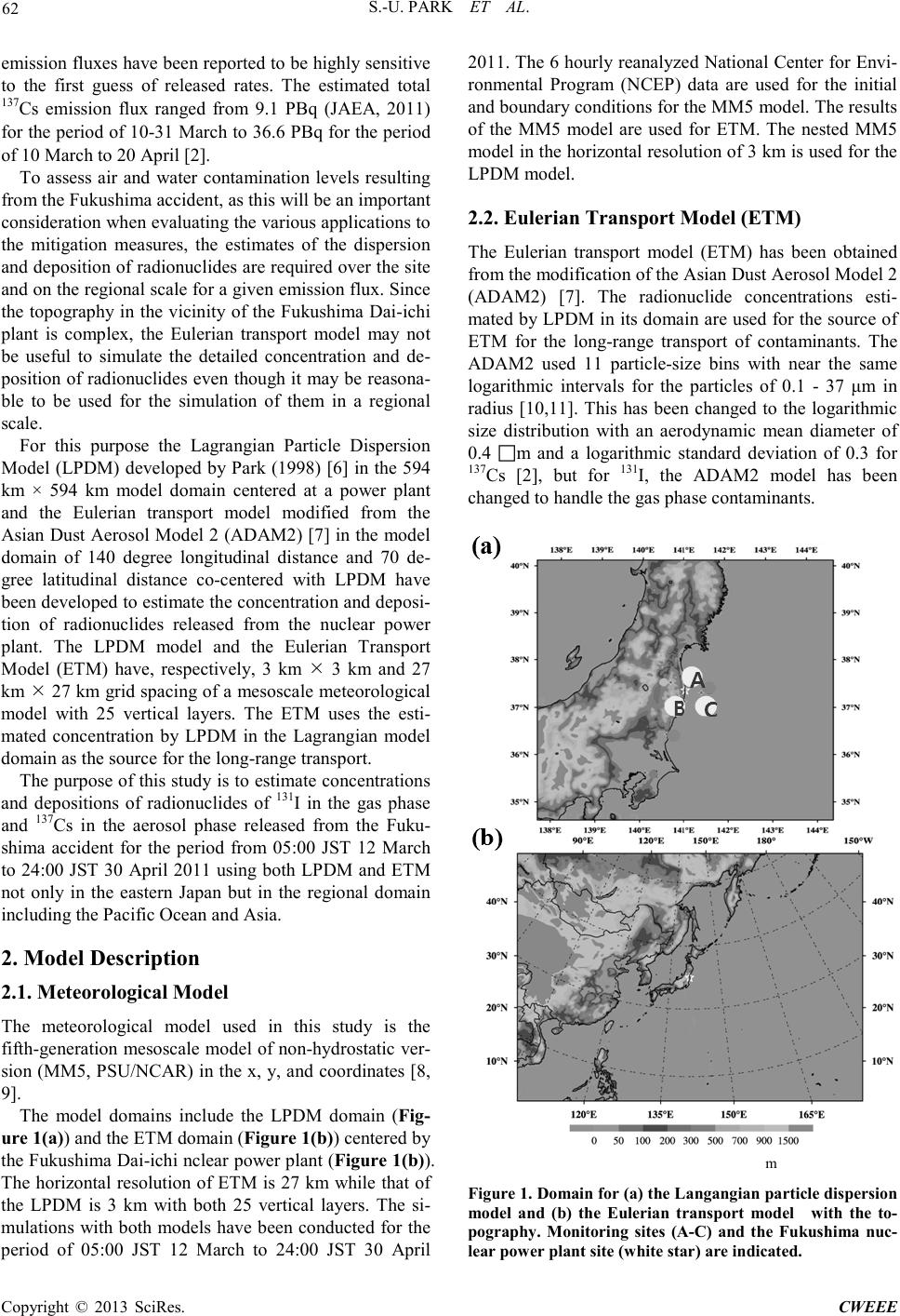

S.-U. PARK ET AL.

emis sion flu xes have b ee n rep or ted t o b e highl y sens iti ve

to the first guess of released rates. The estimated total

137Cs emission flux ranged from 9.1 PBq (JAEA, 2011)

for the period of 10-31 March to 36.6 PBq for the period

of 10 March to 20 April [2].

To assess air and water contamination levels resulting

from the Fukushima accident, as th is will be an important

consideratio n whe n e valuatin g the variou s app licatio ns to

the mitigation measures, the estimates of the dispersion

and deposition of radionuclides are required over the site

and o n the r egio nal sca le fo r a give n e missio n flu x. Si nce

the topography in the vicinity of the Fukushima Dai-ichi

plant is complex, the Eulerian transport model may not

be useful to simulate the detailed concentration and de-

position of radionuclides even though it may be reasona-

ble to be used for the simulation of them in a regional

scale.

For this purpose the Lagrangian Particle Dispersion

Model (LPDM) developed by Park (1998) [6] in the 594

km × 594 km model domain centered at a power plant

and the Eulerian transport model modified from the

Asian D ust Aerosol Model 2 (ADAM2) [7] in the model

domain of 140 degree longitudinal distance and 70 de-

gree latitudinal distance co-centered with LPDM have

been developed to estimate the concentration and deposi-

tion of radionuclides released from the nuclear power

plant. The LPDM model and the Eulerian Transport

Model (ETM) have, respectively, 3 km  3 km and 27

km  27 km grid spacing of a mesoscale meteorological

model with 25 vertical layers. The ETM uses the esti-

mated concentration by LPDM in the Lagrangian model

domain as the source for the long-range transport.

The purp ose of this study is to estimate co ncentrations

and depositions of radionuclides of 131I in the gas phase

and 137Cs in the aerosol phase released from the Fuku-

shima accident for the period from 05:00 JST 12 March

to 24:00 JST 30 April 2011 using both LPDM and ETM

not only in the eastern Japan but in the regional domain

including the Pacific Ocean and Asia.

2. Model Descri ption

2.1. Meteorological Model

The meteorological model used in this study is the

fift h-generation mesoscale model of non-hydrostatic ver-

sion ( MM5, P SU/NCAR ) in the x, y, a nd coordinates [8,

9].

The model domains include the LPDM domain (Fig-

ure 1(a)) and t he ETM domain (Figure 1(b)) centered by

the F ukushi ma Dai -ichi nclear po wer plant (Figure 1(b)).

The horizontal resolution of ETM is 27 km while that of

the LPDM is 3 km with both 25 vertical layers. The si-

mulations with both models have been conducted for the

period of 05:00 JST 12 March to 24:00 JST 30 April

2011. The 6 hourly reanalyzed National Center for Envi-

ronmental Program (NCEP) data are used for the initial

and boundary conditions for the MM5 model. The results

of the MM5 model are used for ETM. The nested MM5

model in the horizontal resolution of 3 km is used for the

LPDM model.

2.2. Eulerian Transport Model (ETM)

The Eulerian transport model (ETM) has been obtained

from the modification of the Asian Dust Aerosol Model 2

(ADAM2) [7]. The radionuclide concentrations esti-

mated by LPDM in its domain are used for the source of

ETM for the long-range transport of contaminants. The

ADAM2 used 11 particle-size bins with near the same

logarithmic intervals for the particles of 0.1 - 37 μm in

radius [10,11]. This has been changed to the logarithmic

size distribution with an aerodynamic mean diameter of

0.4 m and a logarithmic standard deviation of 0.3 for

137Cs [2], but for 131I, the ADAM2 model has been

chan ged to handle the gas p hase contami nants.

Figure 1. Domain for (a) the Langangian particle dispersion

model and (b) the Eulerian transport model with the to-

pography. Monitoring sites (A-C) and the Fukushima nuc-

lear power plant site (whit e star) are in dicated.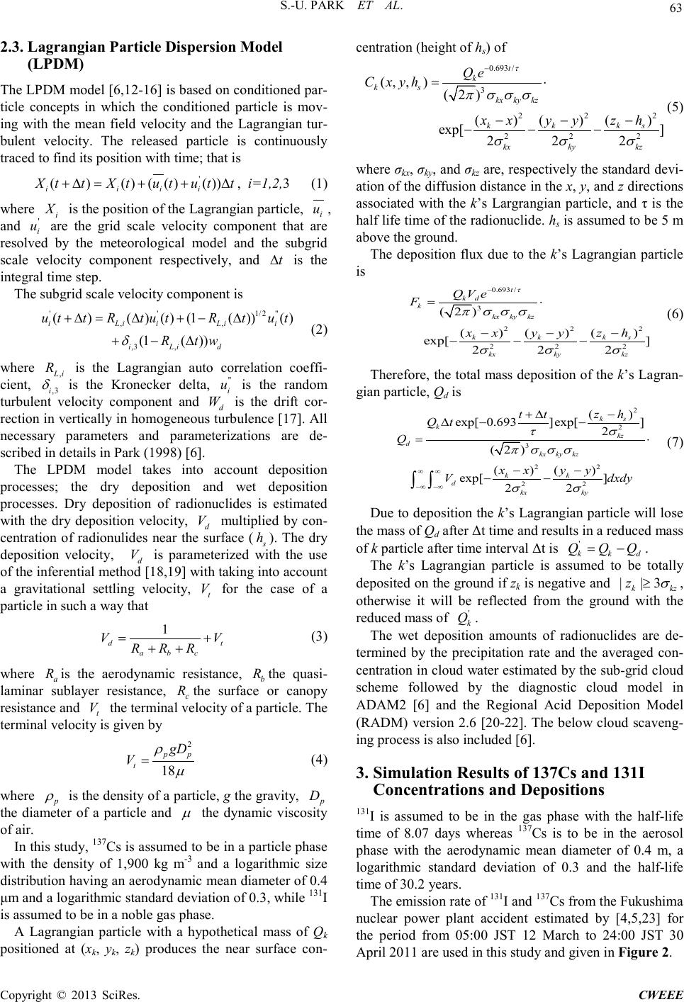

S.-U. PARK ET AL.

2.3. Lagrangian Particle Dispersion Model

(LPDM)

The LPDM model [6,12-16] is based on conditioned par-

ticle concepts in which the conditioned particle is mov-

ing with the mean field velocity and the Lagrangian tur-

bulent velocity. The released particle is continuously

traced to find its position with time; that is

()()( ()())

ii ii

XttXtut utt+∆ =++∆

, i=1,2,3 (1)

where

is the positio n o f the Lagran gian pa rticle,

and

are the grid scale velocity component that are

resolved by the meteorological model and the subgrid

scale velocity component respectively, and

t∆

is the

integral time step.

The subgrid scale velocity component is

''1/2 "

,3 ,

()( )()(1( ))()

(1( ))

iLi iLii

i Li d

uttR tutR tut

R tw

+∆ =∆+−∆

+ −∆

(2)

where ,Li

is the Lagrangian auto correlation coeffi-

cient, ,3i

is the Kronecker delta,

is the random

turbulent velocity component and d

W is the drift cor-

rec tion in vertica lly i n homo geneo us turb ulence [17 ]. All

necessary parameters and parameterizations are de-

scribed in details in Park (1998) [6].

The LPDM model takes into account deposition

processes; the dry deposition and wet deposition

processes. Dry deposition of radionuclides is estimated

with the dry deposition velocity,

multiplied by con-

centration of radionulides near the surface (

). T he dry

deposition velocity,

is parameterized with the use

of the inferential method [18,19] with taking into account

a gravitational settling velocity,

for the case of a

particle i n s uch a wa y that

abc

RRR

= +

(3)

where

is the aerodynamic resistance,

the quasi-

laminar sublayer resistance,

the surface or canopy

resistance and

the terminal velocity of a particle. The

terminal velocit y is given by

(4)

where

is the density of a particle, g t he gra vity, p

the diameter of a particle and

the dynamic viscosity

of air.

In thi s st udy, 137Cs is assumed to be in a particle phase

with the density of 1,900 kg m-3 and a logarithmic size

distribution having an aerodynamic mean diameter of 0.4

μm and a logarithmic standard deviation of 0.3, while 131I

is assumed to be in a noble gas phase.

A Lagrangian particle with a hypothetical mass of Qk

positioned at (xk, yk, zk) produces the near surface con-

centration (he ight of hs) of

0.693 /

22 2

(,, )(2)

( )()()

exp[]

222

kx ky kz

kk ks

kx kykz

C xyh

xxyy zh

π σσσ

σσ σ

−

= ⋅

−−−

−− −

(5)

where σkx, σky, and σkz are, respectively the standard devi-

ation of the diffusio n distance in the x, y, a nd z dire ctions

associated with the k’s Largrangian particle, and τ is the

half life time of the radionuclide. hs is assumed to be 5 m

above the ground.

The deposition flux due to the k’s Lagrangian particle

0.693 /

22 2

(2)

( )()()

exp[ ]

222

kx ky kz

k k ks

kx kykz

QVe

xx yy zh

π σσσ

σσ σ

−

= ⋅

−−−

−− −

(6)

Therefore, the total mass depo sition of t he k’s Lagra n-

gian particle, Qd is

()

exp[ 0.693]exp[]

(2)

( )()

exp[ ]

kx ky kz

kx ky

xx yy

V dxdy

τσ

π σσσ

σσ

∞∞

−∞ −∞

−

+∆

∆− −

= ⋅

−−

∫∫

(7)

Due to depo sition the k’s Lagrangian p article will lose

the mass of Qd after Δt time and results in a reduced mass

of k particle after time interval Δt is

k kd

QQQ= −

The k’s Lagrangian particle is assumed to be totally

deposited on the ground if zk is ne gative and

| |3

k kz

≥

otherwise it will be reflected from the ground with the

reduced mass of

The wet deposition amounts of radionuclides are de-

termined by the precipitation rate and the averaged con-

centration in cloud water estimated by the sub-grid cloud

scheme followed by the diagnostic cloud model in

ADAM2 [6] and the Regional Acid Deposition Model

(RADM) version 2.6 [20-22]. The below cloud scaveng-

ing pr ocess is also inc l uded [6].

3. Simulation Results of 137Cs and 131I

Concentrations and Depositions

131I is assumed to be in the gas phase with the half-life

time of 8.07 days whereas 137Cs is to be in the aerosol

phase with the aerodynamic mean diameter of 0.4 m, a

logarithmic standard deviation of 0.3 and the half-life

time of 30.2 years.

The emission rate of 131I and 137Cs from the Fukushima

nuclear power plant accident estimated by [4,5,23] for

the period from 05:00 JST 12 March to 24:00 JST 30

April 2011 are used in t his study and given in Figure 2 .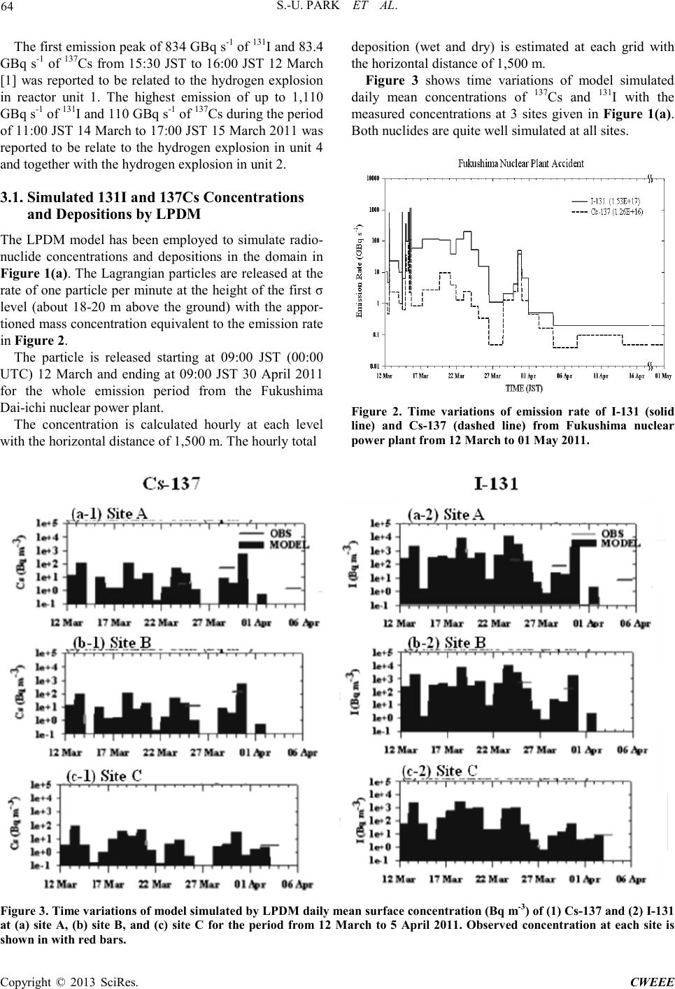

S.-U. PARK ET AL.

The first emission peak of 834 GBq s-1 of 131I and 83.4

GBq s-1 of 137Cs from 15:30 JST to 16:00 JST 12 March

[1] was reported to be related to the hydrogen explosion

in reactor unit 1. The highest emission of up to 1,110

GBq s-1 of 131I and 110 GBq s-1 of 137Cs dur i ng t he p er io d

of 11:00 JST 14 March to 17:00 JST 15 March 2011 was

reported to be relate to the hydrogen explosion in unit 4

and together with the hydrogen explosion in unit 2.

3.1. Simulated 131I and 137Cs Concentrations

and Depositions by LPDM

The LPDM model has been employed to simulate radio-

nuclide concentrations and depositions in the domain in

Figure 1(a). The Lagrangian particles are released at the

rate of one particle per minute at the height of the first σ

level (about 18-20 m above the ground) with the appor-

tioned mass co ncentratio n equivale nt to the e mission rate

in Figure 2.

The particle is released starting at 09:00 JST (00:00

UTC) 12 March and ending at 09:00 JST 30 April 2011

for the whole emission period from the Fukushima

Dai-ichi nuclear power pla nt.

The concentration is calculated hourly at each level

with the horiz ontal d istanc e of 1 ,500 m. The hour ly total

deposition (wet and dry) is estimated at each grid with

the horizontal distance o f 1,500 m.

Figure 3 shows time variations of model simulated

daily mean concentrations of 137Cs and 131I with the

measured concentrations at 3 sites given in Figure 1(a).

Both nuclide s are quite well si mula te d at all site s.

Figure 2. Time variations of emission rate of I-131 (solid

line) and Cs-137 (dashed line) from Fukushima nuclear

pow e r plant from 12 M ar c h to 01 M ay 2011.

Fig ure 3 . T i me varia ti o ns of mode l s i mul at e d by LP DM dai ly mea n su rf ac e c o nce ntr a ti o n (B q m-3) of (1) Cs-137 and (2) I-131

at (a) site A, (b) site B, and (c) site C for the period from 12 March to 5 April 2011. Observed concentration at each site is

shown in wi th red bars .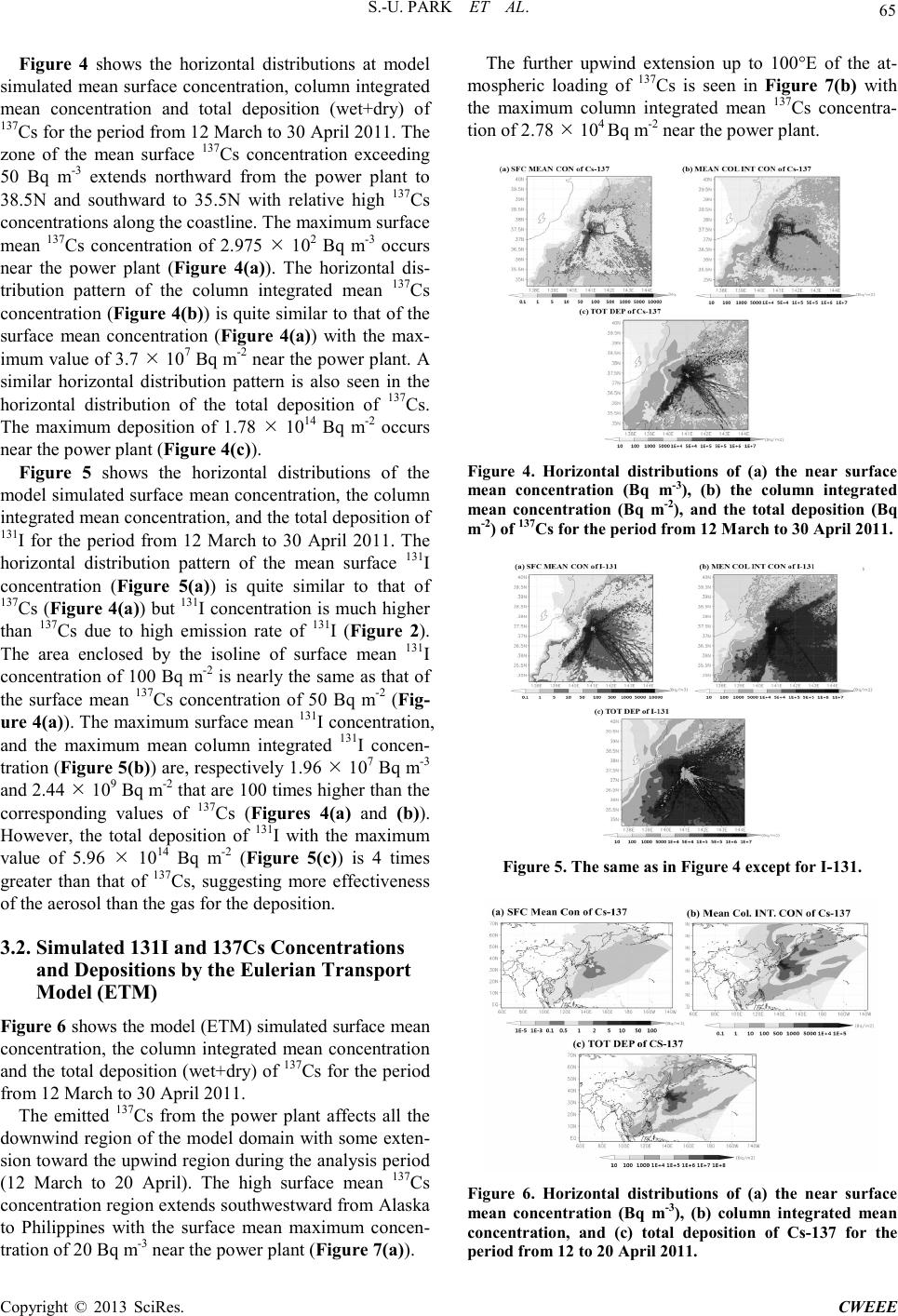

S.-U. PARK ET AL.

Figure 4 shows the horizontal distributions at model

simulated mean surface concentration, column integrated

mean concentration and total deposition (wet+dry) of

137Cs for the period from 12 March to 30 April 2011. The

zone of the mean surface 137Cs concentration exceeding

50 Bq m-3 extends northward from the power plant to

38.5N and southward to 35.5N with relative high 137Cs

concentrations along the coastline. The maximum surface

mean 137Cs concentration of 2.975  102 Bq m-3 occurs

near the power plant (Figure 4(a)). The horizontal dis-

tribution pattern of the column integrated mean 137Cs

concentration (Figure 4(b)) is quite similar to that of the

surface mean concentration (Figure 4(a)) with the max-

imum value of 3.7  107 Bq m-2 near the power plant. A

similar horizontal distribution pattern is also seen in the

horizontal distribution of the total deposition of 137Cs.

The maximum deposition of 1.78  1014 Bq m-2 occurs

near the power plant (Figure 4(c)).

Figure 5 shows the horizontal distributions of the

model simulated surface mean concentration, the column

integrated mean co ncentr ation , and the to tal deposition of

131I for the period from 12 March to 30 April 2011. The

horizontal distribution pattern of the mean surface 131I

concentration (Figure 5(a)) is quite similar to that of

137Cs (Figure 4(a)) but 131I c oncentra tion i s much hi gher

than 137Cs due to high emission rate of 131I (Figure 2).

The area enclosed by the isoline of surface mean 131I

concentratio n of 100 Bq m-2 is nearly the same as that of

the surface mean 137Cs concentration of 50 Bq m-2 (Fig-

ure 4(a)). The maximum surface mean 131I concentration,

and the maximum mean column integrated 131I concen-

tration (Fig ure 5(b)) are, r espectively 1.96  107 Bq m-3

and 2.44  109 Bq m-2 tha t ar e 1 00 times hi ghe r tha n t he

corresponding values of 137Cs (Figures 4(a) and (b)).

However, the total deposition of 131I with the maximum

value of 5.96  1014 Bq m-2 (Figure 5(c)) is 4 times

greater than that of 137Cs, suggesting more effectiveness

of the aerosol than the gas for the deposition.

3.2. Simulated 131I and 137Cs Concentrations

and Depositions by the Eulerian Transport

Model (ETM)

Figure 6 shows the model (ET M) simulated surface mean

concentration, the column integrated mean concentration

and the total dep osition (wet+dry) of 137Cs for the period

from 12 March to 30 April 2011.

The emitted 137Cs from the power plant affects all the

downwind region of the model domain with some exten-

sion to ward the up wind regi on dur ing the anal ysis per iod

(12 March to 20 April). The high surface mean 137Cs

conc ent ra tion r e gio n e xtend s s o uth we st war d from Alas ka

to Philippines with the surface mean maximum concen-

tration of 20 Bq m-3 near the power plant (Figure 7(a)).

The further upwind extension up to 100°E of the at-

mospheric loading of 137Cs is seen in Figure 7(b) with

the maximum column integrated mean 137Cs concentra-

tion of 2.78  104 Bq m-2 near the po wer plant.

Figure 4. Horizontal distributions of (a) the near surface

mean concentration (Bq m-3), (b) the column integrated

mean concentration (Bq m-2), and the total deposition (Bq

m-2) of 137Cs for the period from 12 March to 30 April 2011.

Figure 5 . The same as in Figure 4 except for I-131.

Figure 6. Horizontal distributions of (a) the near surface

mean concentration (Bq m-3), (b) column integrated mean

concentration, and (c) total deposition of Cs-137 for the

period from 12 to 20 April 2011.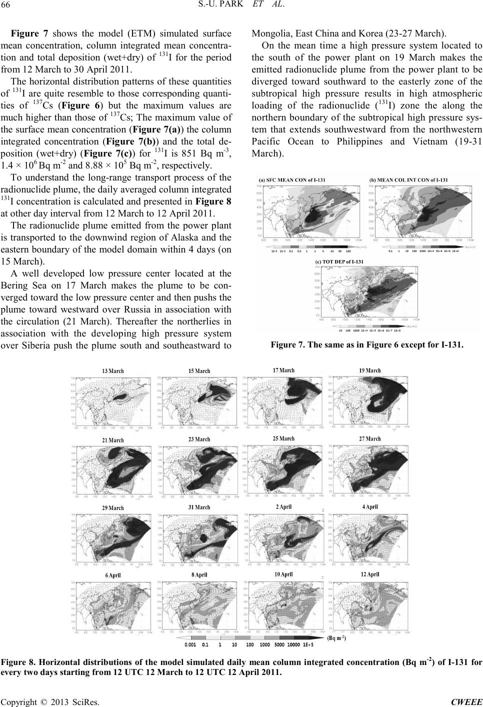

S.-U. PARK ET AL.

Figure 7 shows the model (ETM) simulated surface

mean concentration, column integrated mean concentra-

tion and total deposition (wet+dry) of 131I for the period

from 12 March to 30 April 2011.

The horizontal distribution patterns of these quantities

of 131I are quite resemble to those corresponding quanti-

ties of 137Cs (Figure 6) but the maximum values are

much higher than tho se of 137Cs; The ma ximum va lue of

the surface mean concentration (Figure 7(a)) the column

integrated concentration (Figure 7(b)) and the total de-

position (wet+dry) (Figure 7(c)) for 131I is 851 Bq m-3,

1.4 × 106 Bq m-2 and 8.88 × 105 Bq m-2, respectively.

To understand the long-range transport process of the

radionuclide plume, the daily averaged column integrated

131I concentration is calculated and presented in Figure 8

at other day interval from 12 March to 12 April 2011.

The radionuclide plume emitted from the power plant

is transported to the downwind region of Alaska and the

eastern boundary of the model domain within 4 days (on

15 March).

A well developed low pressure center located at the

Bering Sea on 17 March makes the plume to be con-

verge d to ward the lo w pre ssur e c enter and then pus hs t he

plume toward westward over Russia in association with

the circulation (21 March). Thereafter the northerlies in

association with the developing high pressure system

over Siberia push the plume south and southeastward to

Mongolia, East China and Korea (23-27 March).

On the mean time a high pressure system located to

the south of the power plant on 19 March makes the

emitted radionuclide plume from the power plant to be

diverged toward southward to the easterly zone of the

subtropical high pressure results in high atmospheric

loading of the radionuclide (131I) zone the along the

northern boundary of the subtropical high pressure sys-

tem that extends southwestward from the northwestern

Pacific Ocean to Philippines and Vietnam (19-31

March).

Figure 7 . The same as in Figure 6 except for I-131.

Figure 8. Horizontal distributions of the model si mulated dail y mean colu mn integr ated concentr ation (B q m-2) of I-131 for

every two days starting from 12 UTC 12 March to 12 UTC 12 April 2011.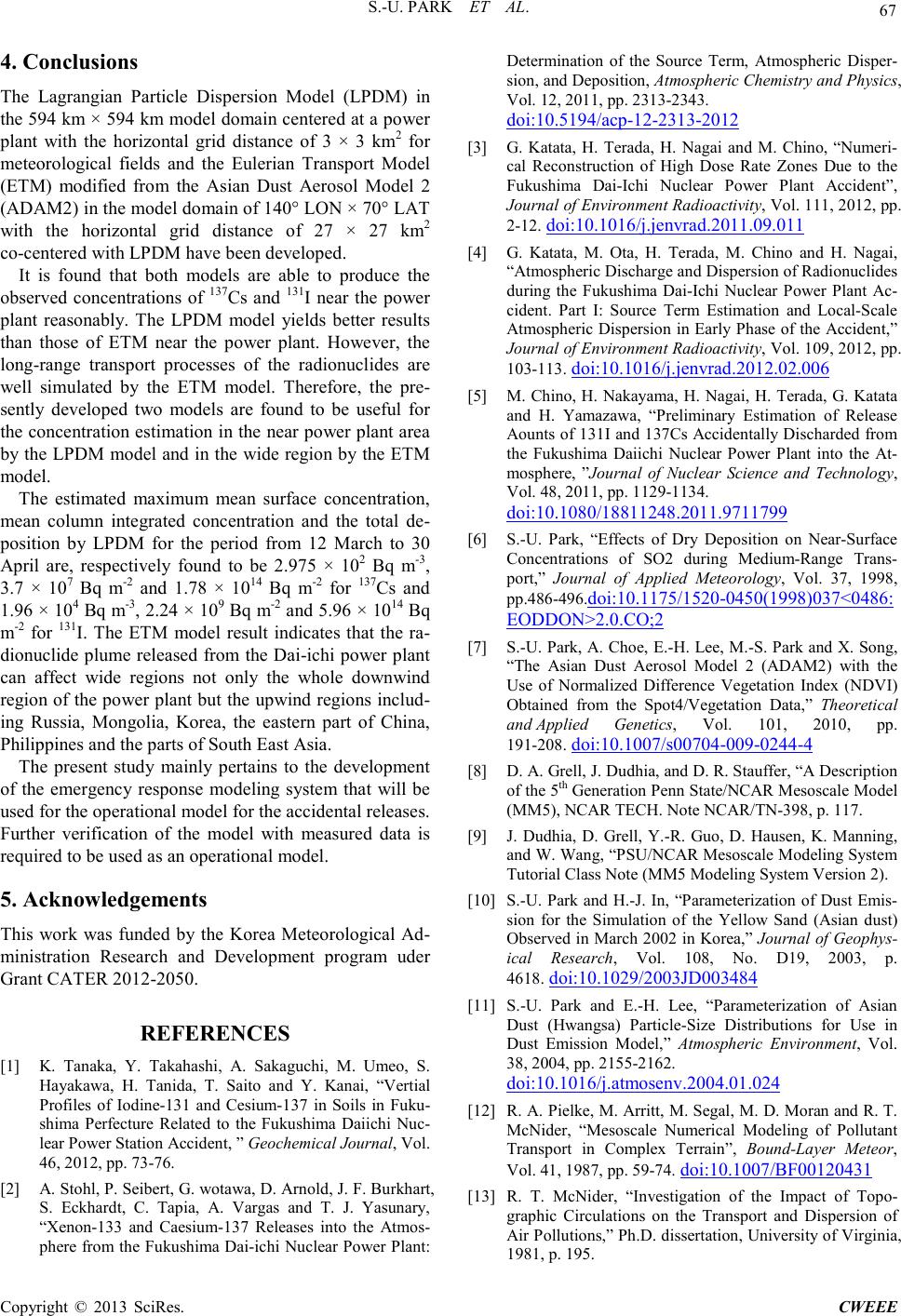

S.-U. PARK ET AL.

4. Conclusions

The Lagrangian Particle Dispersion Model (LPDM) in

the 594 km × 594 km model domain centered at a power

plant with the horizontal grid distance of 3 × 3 km2 for

meteorological fields and the Eulerian Transport Model

(ETM) modified from the Asian Dust Aerosol Model 2

(ADAM2) in the model domain of 140° LON × 70° LAT

with the horizontal grid distance of 27 × 27 km2

co-centered with LPDM have been developed.

It is found that both models are able to produce the

observed concentrations of 137Cs and 131I near the power

plant reasonably. The LPDM model yields better results

than those of ETM near the power plant. However, the

long-range transport processes of the radionuclides are

well simulated by the ETM model. Therefore, the pre-

sently developed two models are found to be useful for

the concentration estimation in the near power plant area

by the LP DM model and i n the wid e regi on by the ETM

model.

The estimated maximum mean surface concentration,

mean column integrated concentration and the total de-

position by LPDM for the period from 12 March to 30

April are, respectively found to be 2.975 × 102 Bq m-3,

3.7 × 107 Bq m-2 and 1.78 × 1014 Bq m-2 for 137Cs and

1.96 × 104 Bq m-3, 2.24 × 109 Bq m-2 and 5.96 × 1014 Bq

m-2 for 131I. The ETM model result indicates that the ra-

dionuclide plume released from the Dai-ichi power plant

can affect wide regions not only the whole downwind

regio n of the p ower p lant but the up wind reg ions incl ud-

ing Russia, Mongolia, Korea, the eastern part of China,

Philippines and the parts of South East Asia.

The present study mainly pertains to the development

of the emergency response modeling system that will be

used for the operational model for the accidental releases.

Further verification of the model with measured data is

required to be used as an operational model.

5. Acknowledgements

This work was funded by the Korea Meteorological Ad-

ministration Research and Development program uder

Grant CATER 2012-2050.

REFERENCES

[1] K. Tanaka, Y. Takahashi, A. Sakaguchi, M. Umeo, S.

Hayakawa, H. Tanida, T. Saito and Y. Kanai, “Vertial

Profiles of Iodine-131 and Cesium-137 in Soils in Fuku-

shima Perfecture Related to the Fukushima Daiichi Nuc-

lear Po wer Statio n Accident , ” Geochemical Journal, Vol.

46, 2012 , pp. 73-76.

[2] A. Stohl, P. Seibert, G. wotawa, D. Arnold, J. F. Burkhart,

S. Eckhardt, C. Tapia, A. Vargas and T. J. Yasunary,

“Xenon-133 and Caesium-137 Releases into the Atmos-

phere from the Fukushima Dai-ichi Nuclear Power Plant:

Determination of the Source Term, Atmospheric Disper-

sion, and Deposition, Atmospheric Chemistry and Physics,

Vol. 12, 2011, pp. 2313-2343.

doi:10.5194/acp-12-2313-2012

[3] G. Katata, H. Terada, H. Nagai and M. Chino, “Numer i-

cal Reconstruction of High Dose Rate Zones Due to the

Fukushima Dai-Ichi Nuclear Power Plant Accident”,

Journal of Environment Radioactivity, Vol. 111, 2012, pp.

2-12. doi:10.1016/j.jenvrad.2011.09.011

[4] G. Katata, M. Ota, H. Terada, M. Chino and H. Nagai,

“Atmospheric Dischar ge and Dispersion of Radionuclides

during the Fukushima Dai-Ichi Nuclear Power Plant Ac-

cident. Part I: Source Term Estimation and Local-Scale

Atmospheric Dispersion in Early Phase of the Accident,”

Journal of Environment Radioactivity, Vol. 109, 2012, pp.

103-113. doi:10.1016/j.jenvrad.2012.02.006

[5] M. Chino, H. Nakayama, H. Nagai, H. Terada, G. Katata

and H. Yamazawa, “Preliminary Estimation of Release

Aounts of 131I and 137Cs Accidentally Di scharded fro m

the Fukushima Daiichi Nuclear Power Plant into the At-

mosphere, ”Journal of Nuclear Science and Technology,

Vol. 48, 2011, pp. 1129-1134.

doi:10.1080/18811248.2011.9711799

[6] S.-U. Park, “Effects of Dry Deposition on Near-Surface

Concentrations of SO2 during Medium-Range Trans-

port,” Journal of Applied Meteorology, Vol. 37, 1998,

pp.486-496.doi:10.1175/1520-0450(1998)037<0486:

EODDON>2.0.CO;2

[7] S.-U. Park, A. Choe, E.-H. Lee, M.-S . Park and X. Song,

“The Asian Dust Aerosol Model 2 (ADAM2) with the

Use of Normalized Difference Vegetation Index (NDVI)

Obtained from the Spot4/Vegetation Data,” Theoret ical

and Applied Genetics, Vol. 101, 2010, pp.

191-208. doi:10.1007/s00704-009-0244-4

[8] D. A. Grell, J. Dudhia, and D. R. Stauffer, “A Description

of the 5th Generati on P enn State/NC AR Mesoscale Model

(MM5), NCAR TECH. Note NCAR/TN-398, p. 117.

[9] J. Dudhia, D. Grell, Y.-R. Guo, D. Hausen, K. Manning,

and W. Wang, “PSU/NCAR Mesoscale Modeling System

Tutorial Class Note (MM5 Modeling System Version 2).

[10] S.-U. P ark and H.-J. In, “Par ameterization of Dust Emis-

sion for the Simulation of the Yellow Sand (Asian dust)

Observed in March 2002 in Korea,” Journal of Geophys-

ical R esearch, Vol. 108, No. D19, 2003, p.

4618. doi:10.1029/2003JD003484

[11] S.-U. Park and E.-H. Lee, “Parameterization of Asian

Dust (Hwangsa) Particle-Size Distributions for Use in

Dust Emission Model,” Atmospheric Environment, Vol.

38, 2004, pp. 2155-2162.

doi:10.1016/j.atmosenv.2004.01.024

[12] R. A. Pielke, M. Arritt, M. Segal, M. D. Moran and R. T.

McNider, “Mesoscale Numerical Modeling of Pollutant

Transport in Complex Terrain”, Bound-Layer Meteor,

Vol. 41, 1987, pp. 59-74. doi:10.1007/BF00120431

[13] R. T. McNider, “Investigation of the Impact of Topo-

graphic Circulations on the Transport and Dispersion of

Air Pollutions,” Ph.D. dissertation, University of Virginia,

1981, p. 195.

S.-U. PARK ET AL.

[14] T. Yamada, J. Kao, and S. Bunker, “Airflow and Air

Quality Simulations over the Western Mountaineous Re-

gion with a Four-Dimensional Data Assimilation Tech-

nique,” Atmospheric Envi r onmen t, Vol.23, 1989,

pp.539-554. doi:10.1016/0004-6981(89)90003-6

[15] W. L. Physick, and D. J. Abbs, “Modeling of Summer-

time Flow and Dispersion in the Coastal Terrain of Sou-

theastern Asutralia,” Monthly Weather Review, Vol.119,

1991,pp.1014-1030. doi:10.1175/1520-0493(1991)11

9<1014:MOSFAD>2.0.CO;2

[16] F. B. Smith, “Conditioned particle motion in a homogen-

ous turbulent field,” Atmospheric Environment, Vol.2,

1968,pp.491-508.doi:10.1016/0004-6981(68)90042-5

[17] B. J. Legg, and M. R. Raupach, “Markov-Chain Simula-

tions of Particle Deposition in Homogeneous Flows: The

Mean Drift Velocity Induced by a Gradient in Eulerian

Velocity Variance”, Bound.-Layer Meteor, Vol.24, 1982,

pp.3-13. doi:10.1007/BF00121796

[18] M. L. Wesely, “Parameterization of Surface Resistances

to Gaseous Dry Deposition in Regional-Scale Numerical

Models,” Atmospheric Environment, Vol.23, 1989,

pp.1293-1304. doi:10.1016/0004-6981(89)90153-4

[19] M. L. Wesel y and B. B. Hicks, “Some Factor s that Affect

the Dispersion Rates of Sulfur Dioxide and Similar Gases

on Vegetation ”, Journal of Air Pollution Control Associ-

ation,Vol.27,1977,pp.1110-1116.

doi:10.1080/00022470.1977.10470534

[20] C. J. Walcek, and G. R. Taylor, “A Theoretical Method

for Computing Vertical Distributions of Acidity and Sul-

fate Production within Cumulus Clouds,” J. Atmos. Sci.,

43,1986,pp.339-355. doi:10.1175/1520-0469(1986)04

3<0339:ATMFCV>2.0.CO;2

[21] J. S. Chang, R. A. Brost, I. S. A. Isaksen, S. Madronich, P.

Middleton, W. R. Stockwell and C. J. Walcek, “A

Three-Dimensional Eulerian Acid Deposition Model:

Physical Concepts and Formulation,” Journal of Geo-

physical Research, Vol. 92, 1987, pp. 14681-14700.

doi:10.1029/JD092iD12p14681

[22] R. L. Dennis, J. N. McHenry, W. R. Barchet, F. S. Bin-

kovski and D. W. Byun, “Correcting RADM’s Sulfate

Underprediction: Discovery and Correction of Model Er-

rors and Testing the Corrections through Comparisons

against Field Dat a,” A tmospheric En vironment, V ol. 27A,

No. 6, 1993, pp. 975-997.

[23] S. Furuta, S. Sumiya, H. Watanabe, M. Nakano, K. Imai-

zumi, M. Takeyasu, A. Nakada, H. Fujita, T. Mizutani, M.

Morisawa, Y. Kokubun, T. Kono, M. Nagaoka, Y. Hiya-

ma, T. Onuma, C. Kato and T. Kurachi, “Results of the

Environmental Radiation Monitoring Following the Ac-

cident at the Fukushima Daiichi Nuclear Power Plant ,”

JAEA-Review, Vol. 035, 2011, p. 89.