Analytical expression of non steady-state concentration profiles at planar electrode for the CE mechanism

doi:10.4236/ns.2010.211160

Vol.2, No.11, 1318-1325 (2010) Natural Science

http://dx.doi.org/10.4236/ns.2010.211160

Analytical expression of non steady-state concentration

profiles at planar electrode for the CE mechanism

Vincent Michael Raj Margret PonRani, Lakshmanan Rajendren

Department of Mathematics, The Madura College, Madurai, India; [email protected]

Received 3 August 2010; revised 5 September 2010; accepted 8 September 2010.

ABSTRACT

The analytical solutions of the non-steady-state

concentrations of species at a planar micro-

electrode are presented. These simple new ap-

proximate expressions of concentrations are

valid for all values of time and possible values

of rate constants. Analytical equations are given

to describe the current when the homogeneous

equilibrium position lies heavily in favour of the

electroinactive species. Working surfaces are

presented for the variation of limiting current

with a homogeneous kinetic parameter and

equilibrium constant. Moreover, in this work we

employ the Homotopy perturbation method to

solve the boundary value problem.

Keywords: Planar Electrode; CE Mechanism;

Mathematical Modelling; Reaction/Diffusion

Equation; Homotopy Perturbation Method

1. INTRODUCTION

One of the major achievements in electroanalytical

chemistry in the 1980s was the introduction of micro-

electrodes, i.e., electrodes whose characteristic dimen-

sion is on the order of a few m



(the radius in the case

of disc and hemispheres, band width in the case of bands,

etc.). Microelectrodes have become more commonly

used in electrochemistry to probe kinetics of fast chemi-

cal reactions [1]. In this work, we are interested in find-

ing the mass transport limiting current response for the

CE mechanism at a microelectrode. For each mechanism,

the electroinactive species A is in dynamic equilibrium

with the electroactive species B via a homogeneous

chemical step. The decay of species A is described by

the first order forward rate constant

f

k and the reverse

of this process is described by the rate constant b

k,

which is first order for the CE mechanism. All species

are considered to have an diffusion coefficient D.

Oldham [2] made use of an analytical expression of

CE mechanism at a hemispherical electrode. Lavagnini

et al .[3] employed the hopscotch method and a confor-

mal map to numerically simulate CE mechanism at a

planar electrode. Values of limiting current were ana-

lysed for a range of equilibrium constants and rate con-

stants. There have been many previous theoretical de-

scriptions of the diffusion limiting current for the CE

mechanism. In Reference [4], Fleischmann et al. dem-

onstrate that Neumann’s integral theorem can be used to

simulate CE mechanism at a disc electrode. However, to

the best of the author’s knowledge, no purely analytical

expressions for the non-steady-state concentrations of

these CE mechanisms have been reported. The purpose

of this communication is to derive approximate analyti-

cal expressions for the non-steady-state concentrations

of the species for all values of 1

m, 2

m, 1

k, 2

k, 3

k

and 4

k using Homotopy perturbation method.

2. MATHEMATICAL FORMULATION OF

THE BOUNDARY VALUE PROBLEM

As a representative example of the reaction-diffusion

problems considered, the standard CE mechanism

2

A

B B eproducts





has been chosen, with initial and boundary conditions

corresponding to the potential step for all planar elec-

trodes. Under stead-state conditions, the local concentra-

tions of the species do not change. Therefore the mass

transport equations are set equal to zero. We consider the

differential equations with diffusion described by the

concentration of the two species leads to the following

equations [5]

2

20

fb

aa

Dkakb

tx







 (1)

2

20

fb

bb

Dkakb

tx







 (2)

where a and b denote the concentration of the spe-

cies

A

and B. x and t stand for space and time, respec-

tively.

f



and b



are described the forward and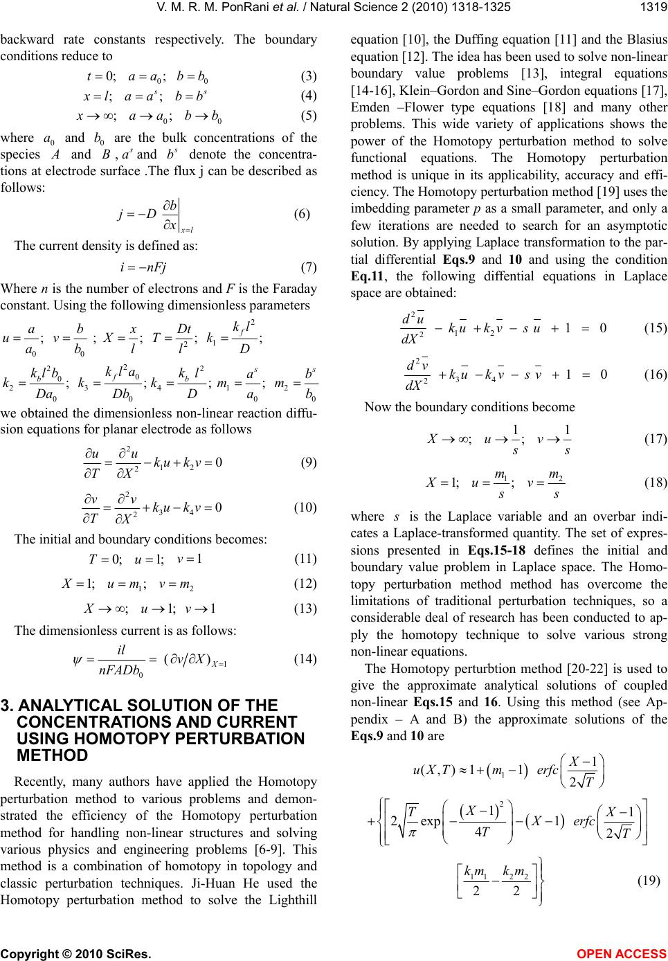

V. M. R. M. PonRani et al. / Natural Science 2 (2010) 1318-1325

1319

backward rate constants respectively. The boundary

conditions reduce to

00

0; ; taabb  (3)

; ;

s

x

laabb 

(4)

00

; ;

x

aabb (5)

where 0

a and 0

b are the bulk concentrations of the

species

A

and B,

s

aand

s

b denote the concentra-

tions at electrode surface .The flux j can be described as

follows:

jD

x

l

b

x





 (6)

The current density is defined as:

inFj (7)

Where n is the number of electrons and F is the Faraday

constant. Using the following dimensionless parameters

2

1

2

00

2

22

0

23412

00 00

; ; ; ; ;

; ; ; ;

f

s

f

bb

kl

ab xDt

uvXT k

ab lD

l

kla

klbk lab

kkkmm

DaDbD ab

 



we obtained the dimensionless non-linear reaction diffu-

sion equations for planar electrode as follows

2

12

20

uu

kuk v

TX





 (9)

2

34

20

vv

ku kv

TX





 (10)

The initial and boundary conditions becomes:

0; 1;Tu



1v (11)

12

1; ;

X

um vm  (12)

; 1; 1Xuv (13)

The dimensionless current is as follows:

1

0

()

X

il vX

nFADb





 (14)

3. ANALYTICAL SOLUTION OF THE

CONCENTRATIONS AND CURRENT

USING HOMOTOPY PERTURBATION

METHOD

Recently, many authors have applied the Homotopy

perturbation method to various problems and demon-

strated the efficiency of the Homotopy perturbation

method for handling non-linear structures and solving

various physics and engineering problems [6-9]. This

method is a combination of homotopy in topology and

classic perturbation techniques. Ji-Huan He used the

Homotopy perturbation method to solve the Lighthill

equation [10], the Duffing equation [11] and the Blasius

equation [12]. The idea has been used to solve non-linear

boundary value problems [13], integral equations

[14-16], Klein–Gordon and Sine–Gordon equations [17],

Emden –Flower type equations [18] and many other

problems. This wide variety of applications shows the

power of the Homotopy perturbation method to solve

functional equations. The Homotopy perturbation

method is unique in its applicability, accuracy and effi-

ciency. The Homotopy perturbation method [19] uses the

imbedding parameter p as a small parameter, and only a

few iterations are needed to search for an asymptotic

solution. By applying Laplace transformation to the par-

tial differential Eqs.9 and 10 and using the condition

Eq.11, the following diffential equations in Laplace

space are obtained:

2

12

2 1 0

du kuk vsu

dX   (15)

2

34

2 1 0

dv ku kvsv

dX



  (16)

Now the boundary conditions become

11

; ; Xuv

s

 (17)

12

1; ;

mm

Xu v

s

 

(18)

where

s

is the Laplace variable and an overbar indi-

cates a Laplace-transformed quantity. The set of expres-

sions presented in Eqs.15-18 defines the initial and

boundary value problem in Laplace space. The Homo-

topy perturbation method method has overcome the

limitations of traditional perturbation techniques, so a

considerable deal of research has been conducted to ap-

ply the homotopy technique to solve various strong

non-linear equations.

The Homotopy perturbtion method [20-22] is used to

give the approximate analytical solutions of coupled

non-linear Eqs.15 and 16. Using this method (see Ap-

pendix – A and B) the approximate solutions of the

Eqs.9 and 10 are



1

(,)11 2

X

uXTmerfc T





 





2

11

2exp1

42

X

TX

Xerfc

TT















































112 2

22

kmk m

















(19)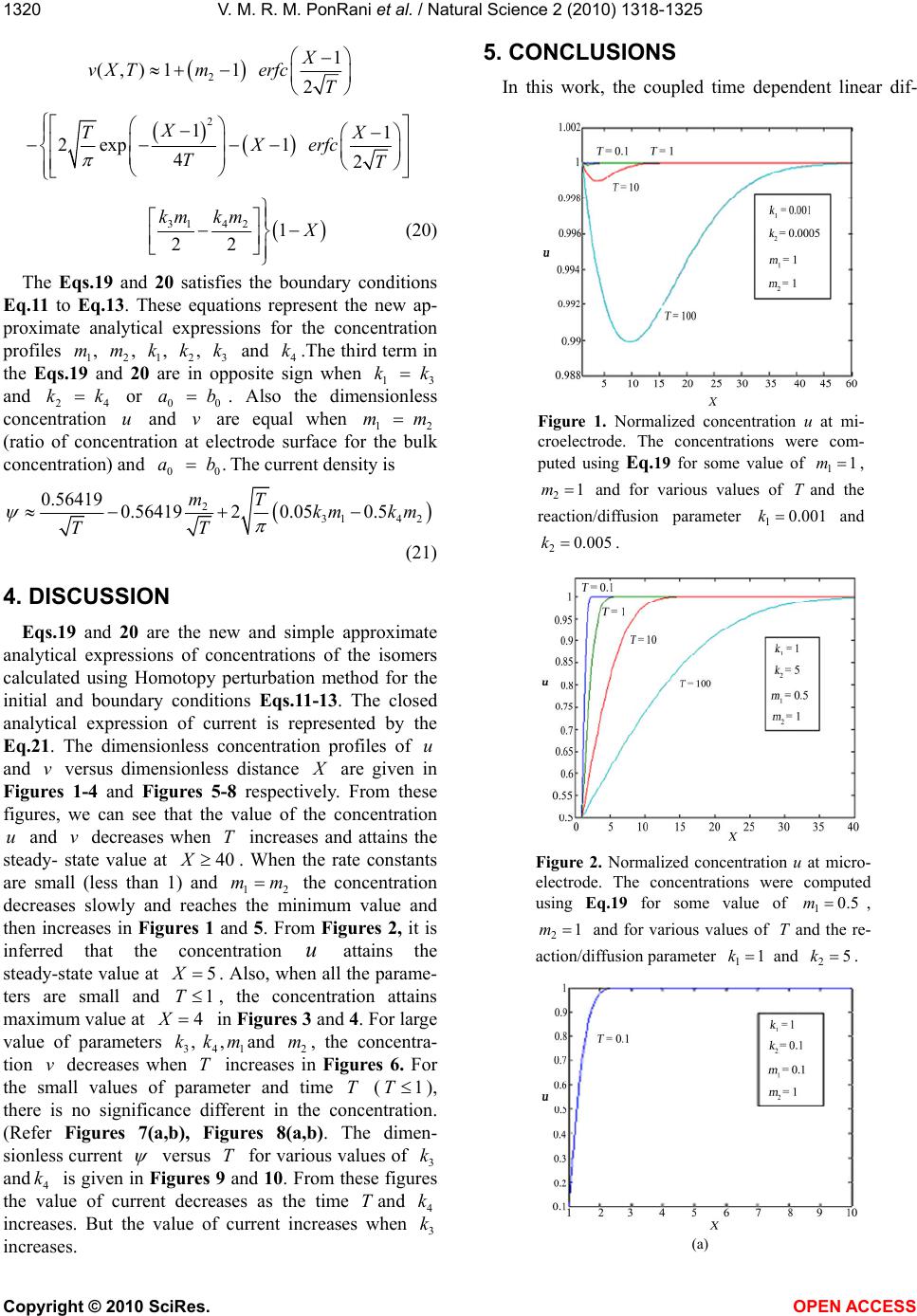

V. M. R. M. PonRani et al. / Natural Science 2 (2010) 1318-1325

1320



2

1

(,)11 2

X

vXTmerfc T





 





2

11

2exp1

42

X

TX

X

erfc

TT

































31 42 1

22

km km X



















(20)

The Eqs.19 and 20 satisfies the boundary conditions

Eq.11 to Eq.13. These equations represent the new ap-

proximate analytical expressions for the concentration

profiles 12123

, , , , mmkk k and 4

k.The third term in

the Eqs.19 and 20 are in opposite sign when 13

kk



and 24

kk or 00

ab. Also the dimensionless

concentration u and v are equal when 12

mm



(ratio of concentration at electrode surface for the bulk

concentration) and 00

.abThe current density is



2

3142

0.56419 0.564192 0.050.5

mTkm km

TT



 

(21)

4. DISCUSSION

Eqs.19 and 20 are the new and simple approximate

analytical expressions of concentrations of the isomers

calculated using Homotopy perturbation method for the

initial and boundary conditions Eqs.11-13. The closed

analytical expression of current is represented by the

Eq.21. The dimensionless concentration profiles of u

and v versus dimensionless distance

X

are given in

Figures 1-4 and Figures 5-8 respectively. From these

figures, we can see that the value of the concentration

u and v decreases when T increases and attains the

steady- state value at 40X. When the rate constants

are small (less than 1) and 12

mm the concentration

decreases slowly and reaches the minimum value and

then increases in Figures 1 and 5. From Figures 2, it is

inferred that the concentration u attains the

steady-state value at 5X. Also, when all the parame-

ters are small and 1T, the concentration attains

maximum value at 4

X

 in Figures 3 and 4. For large

value of parameters 341

, ,kkmand 2

m, the concentra-

tion v decreases when T increases in Figures 6. For

the small values of parameter and time T (1T



),

there is no significance different in the concentration.

(Refer Figures 7(a,b), Figures 8(a,b). The dimen-

sionless current



versus T for various values of 3

k

and 4

k is given in Figures 9 and 10. From these figures

the value of current decreases as the time Tand 4

k

increases. But the value of current increases when 3

k

increases.

5. CONCLUSIONS

In this work, the coupled time dependent linear dif-

Figure 1. Normalized concentration u at mi-

croelectrode. The concentrations were com-

puted using Eq.19 for some value of 11m



,

21m



and for various values of Tand the

reaction/diffusion parameter 10.001 kand

20.005k



.

Figure 2. Normalized concentration u at micro-

electrode. The concentrations were computed

using Eq.19 for some value of 10.5m,

21m



and for various values of Tand the re-

action/diffusion parameter 11 kand 25k



.

(a)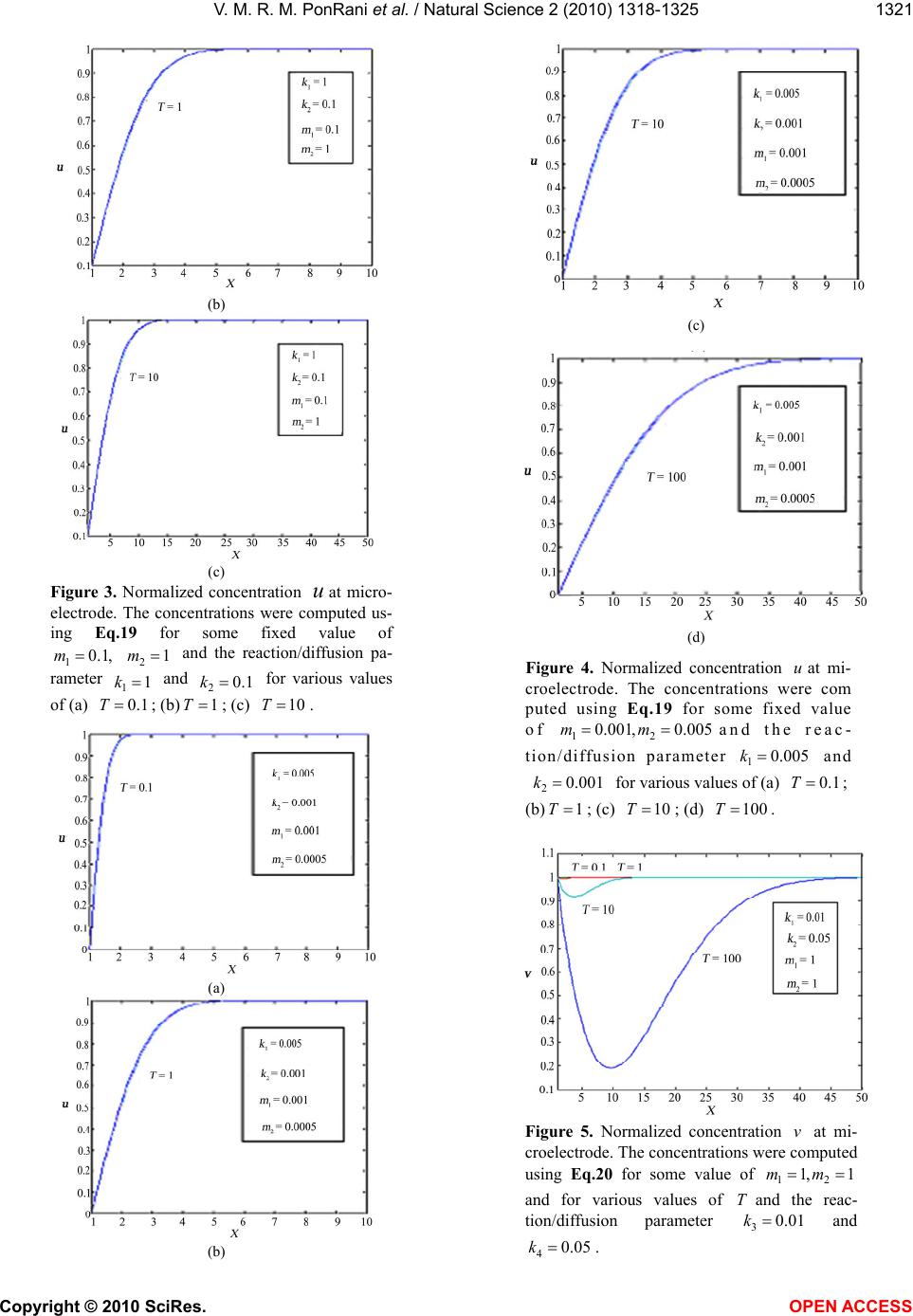

V. M. R. M. PonRani et al. / Natural Science 2 (2010) 1318-1325

1321

(b)

(c)

Figure 3. Normalized concentration uat micro-

electrode. The concentrations were computed us-

ing Eq.19 for some fixed value of

12

0.1, 1mm

and the reaction/diffusion pa-

rameter 11k and 20.1k for various values

of (a) 0.1T; (b)1T; (c) 10T.

(a)

(b)

(c)

(d)

Figure 4. Normalized concentration uat mi-

croelectrode. The concentrations were com

puted using Eq.19 for some fixed value

of 12

0.001,0.005mm



and the reac-

tion/diffusion parameter 10.005k and

20.001k



for various values of (a) 0.1T;

(b) 1T



; (c) 10T



; (d) 100T.

Figure 5. Normalized concentration v at mi-

croelectrode. The concentrations were computed

using Eq.20 for some value of 12

1, 1mm

and for various values of Tand the reac-

tion/diffusion parameter 30.01 kand

40.05k.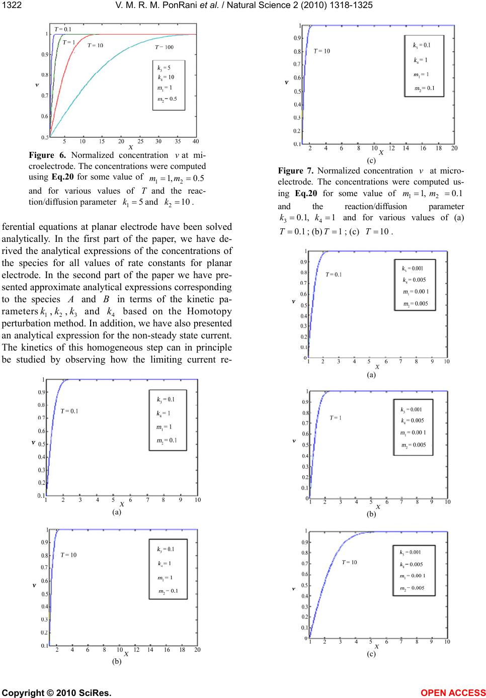

V. M. R. M. PonRani et al. / Natural Science 2 (2010) 1318-1325

1322

Figure 6. Normalized concentration vat mi-

croelectrode. The concentrations were computed

using Eq.20 for some value of 12

1, 0.5mm

and for various values of Tand the reac-

tion/diffusion parameter 15kand 210k.

ferential equations at planar electrode have been solved

analytically. In the first part of the paper, we have de-

rived the analytical expressions of the concentrations of

the species for all values of rate constants for planar

electrode. In the second part of the paper we have pre-

sented approximate analytical expressions corresponding

to the species

A

and B in terms of the kinetic pa-

rameters1

k,2

k,3

k and 4

k based on the Homotopy

perturbation method. In addition, we have also presented

an analytical expression for the non-steady state current.

The kinetics of this homogeneous step can in principle

be studied by observing how the limiting current re-

(a)

(b)

(c)

Figure 7. Normalized concentration v at micro-

electrode. The concentrations were computed us-

ing Eq.20 for some value of 12

1, 0.1mm

and the reaction/diffusion parameter

34

0.1, 1kk



 and for various values of (a)

0.1

T



; (b)1T



; (c) 10T.

(a)

(b)

(c)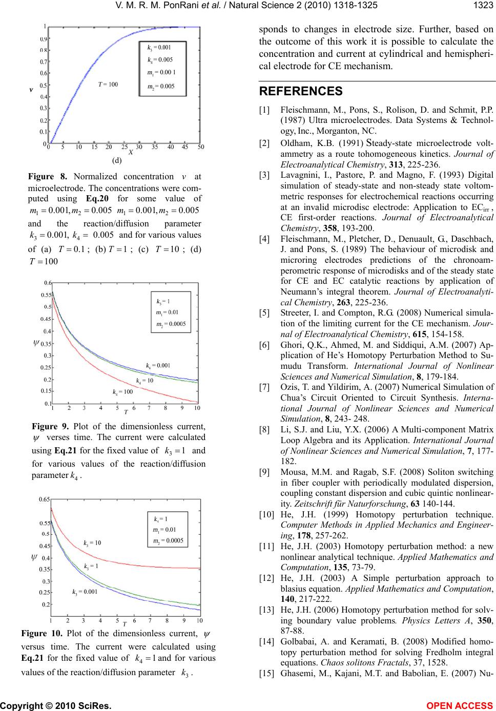

V. M. R. M. PonRani et al. / Natural Science 2 (2010) 1318-1325

1323

(d)

Figure 8. Normalized concentration v at

microelectrode. The concentrations were com-

puted using Eq.20 for some value of

12

0.001,0.005mm

12

0.001,0.005mm



and the reaction/diffusion parameter

34

0.001, 0.005 kkand for various values

of (a) 0.1

T; (b)1T; (c) 10T; (d)

100

T

Figure 9. Plot of the dimensionless current,



verses time. The current were calculated

using Eq.21 for the fixed value of 31k and

for various values of the reaction/diffusion

parameter 4

k.

Figure 10. Plot of the dimensionless current,



versus time. The current were calculated using

Eq.21 for the fixed value of 41kand for various

values of the reaction/diffusion parameter 3

k.

sponds to changes in electrode size. Further, based on

the outcome of this work it is possible to calculate the

concentration and current at cylindrical and hemispheri-

cal electrode for CE mechanism.

REFERENCES

[1] Fleischmann, M., Pons, S., Rolison, D. and Schmit, P.P.

(1987) Ultra microelectrodes. Data Systems & Technol-

ogy, Inc., Morganton, NC.

[2] Oldham, K.B. (1991) Steady-state microelectrode volt-

ammetry as a route tohomogeneous kinetics. Journal of

Electroanalytical Chemistry, 313, 225-236.

[3] Lavagnini, I., Pastore, P. and Magno, F. (1993) Digital

simulation of steady-state and non-steady state voltom-

metric responses for electrochemical reactions occurring

at an invalid microdisc electrode: Application to ECirr ,

CE first-order reactions. Journal of Electroanalytical

Chemistry, 358, 193-200.

[4] Fleischmann, M., Pletcher, D., Denuault, G., Daschbach,

J. and Pons, S. (1989) The behaviour of microdisk and

microring electrodes predictions of the chronoam-

perometric response of microdisks and of the steady state

for CE and EC catalytic reactions by application of

Neumann’s integral theorem. Journal of Electroanalyti-

cal Chemistry, 263, 225-236.

[5] Streeter, I. and Compton, R.G. (2008) Numerical simula-

tion of the limiting current for the CE mechanism. Jour-

nal of Electroanalytical Chemistry, 615, 154-158.

[6] Ghori, Q.K., Ahmed, M. and Siddiqui, A.M. (2007) Ap-

plication of He’s Homotopy Perturbation Method to Su-

mudu Transform. International Journal of Nonlinear

Sciences and Numerical Simulation, 8, 179-184.

[7] Ozis, T. and Yildirim, A. (2007) Numerical Simulation of

Chua’s Circuit Oriented to Circuit Synthesis. Interna-

tional Journal of Nonlinear Sciences and Numerical

Simulation, 8, 243- 248.

[8] Li, S.J. and Liu, Y.X. (2006) A Multi-component Matrix

Loop Algebra and its Application. International Journal

of Nonlinear Sciences and Numerical Simulation, 7, 177-

182.

[9] Mousa, M.M. and Ragab, S.F. (2008) Soliton switching

in fiber coupler with periodically modulated dispersion,

coupling constant dispersion and cubic quintic nonlinear-

ity. Zeitschrift für Naturforschung, 63 140-144.

[10] He, J.H. (1999) Homotopy perturbation technique.

Computer Methods in Applied Mechanics and Engineer-

ing, 178, 257-262.

[11] He, J.H. (2003) Homotopy perturbation method: a new

nonlinear analytical technique. Applied Mathematics and

Computation, 135, 73-79.

[12] He, J.H. (2003) A Simple perturbation approach to

blasius equation. Applied Mathematics and Computation,

140, 217-222.

[13] He, J.H. (2006) Homotopy perturbation method for solv-

ing boundary value problems. Physics Letters A, 350,

87-88.

[14] Golbabai, A. and Keramati, B. (2008) Modified homo-

topy perturbation method for solving Fredholm integral

equations. Chaos solitons Fractals, 37, 1528.

[15] Ghasemi, M., Kajani, M.T. and Babolian, E. (2007) Nu-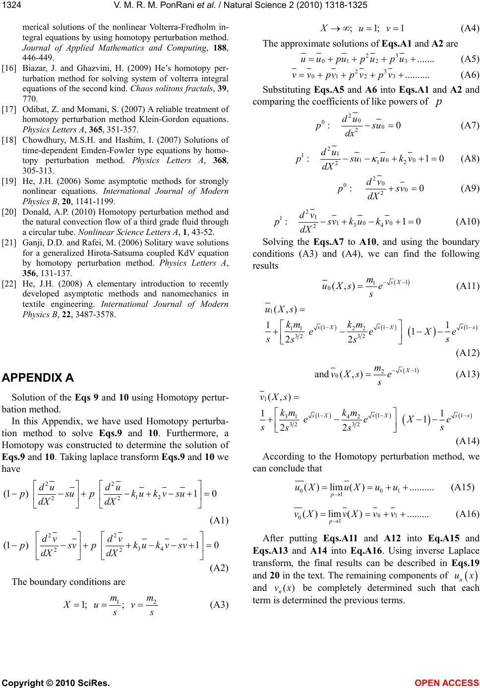

V. M. R. M. PonRani et al. / Natural Science 2 (2010) 1318-1325

1324

merical solutions of the nonlinear Volterra-Fredholm in-

tegral equations by using homotopy perturbation method.

Journal of Applied Mathematics and Computing, 188,

446-449.

[16] Biazar, J. and Ghazvini, H. (2009) He’s homotopy per-

turbation method for solving system of volterra integral

equations of the second kind. Chaos solitons fractals, 39,

770.

[17] Odibat, Z. and Momani, S. (2007) A reliable treatment of

homotopy perturbation method Klein-Gordon equations.

Physics Letters A, 365, 351-357.

[18] Chowdhury, M.S.H. and Hashim, I. (2007) Solutions of

time-dependent Emden-Fowler type equations by homo-

topy perturbation method. Physics Letters A, 368,

305-313.

[19] He, J.H. (2006) Some asymptotic methods for strongly

nonlinear equations. International Journal of Modern

Physics B, 20, 1141-1199.

[20] Donald, A.P. (2010) Homotopy perturbation method and

the natural convection flow of a third grade fluid through

a circular tube. Nonlinear Science Letters A, 1, 43-52.

[21] Ganji, D.D. and Rafei, M. (2006) Solitary wave solutions

for a generalized Hirota-Satsuma coupled KdV equation

by homotopy perturbation method. Physics Letters A,

356, 131-137.

[22] He, J.H. (2008) A elementary introduction to recently

developed asymptotic methods and nanomechanics in

textile engineering. International Journal of Modern

Physics B, 22, 3487-3578.

APPENDIX A

Solution of the Eqs 9 and 10 using Homotopy pertur-

bation method.

In this Appendix, we have used Homotopy perturba-

tion method to solve Eqs.9 and 10. Furthermore, a

Homotopy was constructed to determine the solution of

Eqs.9 and 10. Taking laplace transform Eqs.9 and 10 we

have

22

12

22

(1) 10

du du

psupkukvsu

dX dX

 



 

 

(A1)

22

34

22

(1) 10

dv dv

psvpkukvsv

dX dX

 



 

 

(A2)

The boundary conditions are

12

1; ;

mm

Xu v

s

  (A3)

; 1; 1Xuv (A4)

The approximate solutions of Eqs.A1 and A2 are

23

01 2 3

.......uupu pupu  (A5)

23

01 2 3

..........vvpvpvpv  (A6)

Substituting Eqs. A5 and A6 into Eqs.A1 and A2 and

comparing the coefficients of like powers of p

20

00

2

: 0

du

psu

dx  (A7)

21

1100

12

2

: 10

du

psuukv

dX





 (A8)

20

00

2

: 0

dv

psv

dX  (A9)

21

1100

34

2

: 10

dv

psvkukv

dX



 (A10)

Solving the Eqs. A7 to A10, and using the boundary

conditions (A3) and (A4), we can find the following

results



1

0(,) sX

m

uXs e

s



 (A11)

 



1

11 1

112 2

32 32

(,)

11

1

22

s

XsX sx

uXs

kmk m

eeXe

ss









 





(A12)

and



1

2

0(,) sX

m

vXs e

s



 (A13)

 



1

11 1

31 42

32 32

(,)

11

1

22

s

XsX sx

vXs

km km

eeXe

ss









 





(A14)

According to the Homotopy perturbation method, we

can conclude that

001

1

( )lim()..........

p

uXuXuu



 (A15)

01

( )lim().........

p

vXvXvv



 (A16)

After putting Eqs.A11 and A12 into Eq.A15 and

Eqs.A13 and A14 into Eq.A16. Using inverse Laplace

transform, the final results can be described in Eqs.19

and 20 in the text. The remaining components of





n

ux

and ()

n

vx

be completely determined such that each

term is determined the previous terms.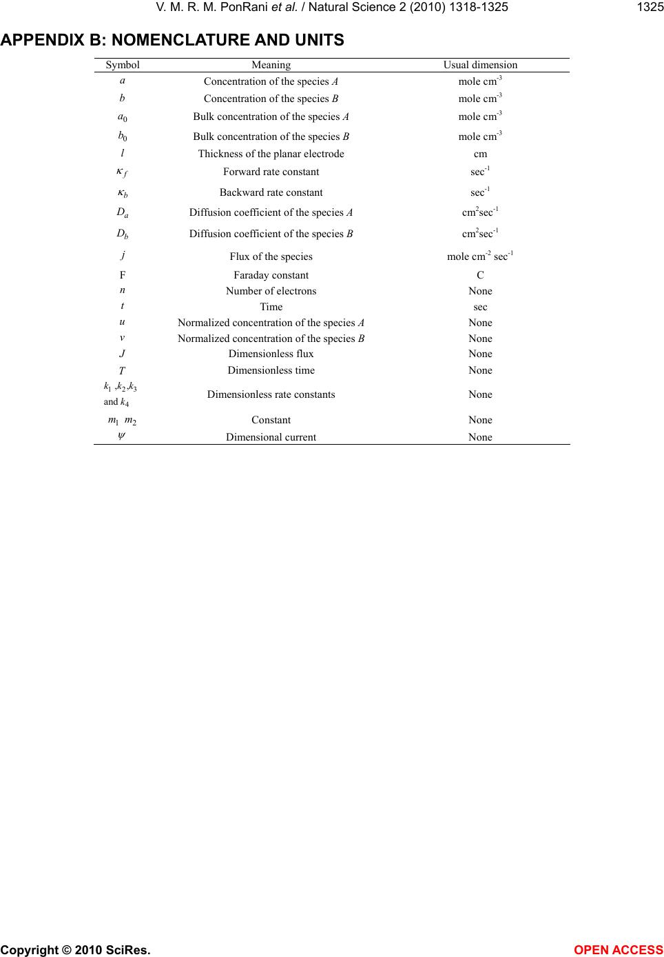

V. M. R. M. PonRani et al. / Natural Science 2 (2010) 1318-1325

1325

APPENDIX B: NOMENCLATURE AND UNITS

Symbol Meaning Usual dimension

a Concentration of the species A mole cm-3

b Concentration of the species B mole cm-3

0

a Bulk concentration of the species A mole cm-3

0

b Bulk concentration of the species B mole cm-3

l Thickness of the planar electrode cm

f



Forward rate constant sec-1

b



Backward rate constant sec-1

a

D

Diffusion coefficient of the species A cm2sec-1

b

D

Diffusion coefficient of the species B cm2sec-1

j Flux of the species mole cm-2 sec-1

F Faraday constant C

n Number of electrons None

t Time sec

u Normalized concentration of the species A None

v Normalized concentration of the species B None

J

Dimensionless flux None

T Dimensionless time None

123

4

,,

and

kkk

k Dimensionless rate constants None

1

m2

m Constant None



Dimensional current None

Paper Menu >>

Journal Menu >>