Research and Analysis of Structural Hole and Matching Coefficient

doi:10.4236/jsea.2010.311127

Paper Menu >>

Journal Menu >>

J. Software Engineering & Applications, 2010, 3, 1080-1087

doi:10.4236/jsea.2010.311127 Published Online November 2010 ( ht t p : / /www.SciRP.org/journal/jsea)

Research and Analysis of Structural Hole and

Matching Coefficient

Penghua Cai, Hai Zhao, Hong Liu, Rong Pan, Zheng Liu, Hui Li

Department of Information Science and Engineeri n g , Northeast University, Shenyang, China.

Email: [email protected]

Received August 28th, 2010; revised September 18th, accepted September 23rd, 2010.

ABSTRACT

Measure is a map from the reality or experimental world to the mathematical world, through which people can more

easily understand the properties of entities and the relationship between them. But the traditional software measure-

ment methods have been unable to effectively measure this large-scale software. Therefore, trustworthy measurement

gives an accurate measurement to these emerging features, providing valuable perspectives and different research di-

mensions to understand software systems. The paper introduces the complex network theory to software measurement

methods and proposes a statistical measurement methodology. First we study the basic parameters of the complex net-

work, and then introduce two new measur ement parameters: structural holes, matching coefficient.

Keywords: Large-Scale Software, Trustworthy Measurement, Structural Holes, Matching Coefficient

1. Introduction

Now large software network is increasingly showing

“small world” and “scale-free”-characteristics of com-

plex networks. The results of studying complex networks

provide strong support for people to explore characteris-

tics of the overall structure of large-scale software net-

work [1,2]. Using a network view research the software

network, this has been recognized by more and more

researchers. The traditional measurement methods focus

on the micro-level statistics and only do some aspects of

the software evaluation because of lacking parameters.

Therefore, the paper imports complex network theory

into the traditional measurement methods and introduces

some new metrics to measure the different characteristics

of the software from the different levels. This paper also

puts forward a measurement methodology, which make

the basic intrinsic property and the overall measures

properties of software as the core and use multiple meas-

urement parameters (the basic parameters in complex

network, the newly introduced metric) to measure some

important characteristics and structural features, provid-

ing an importan t basis for measuring software quality.

2. Structural Hole

1) The theory of structural hole

The concept of structural holes is from the social

structure of competition [3]. It is form social network

research. In brief, structural holes are the relationship

between the two non-duplicate persons. In Figure 1, we

use software network formed by four nodes A, B, C, D to

illustrate structural hole. In the left picture A has three

structural holes (BC, BD and CD); because the three

nodes B, C, D have no direct connection and only node

A is associated with these three classes. Compared with

other three nodes, node A has competitive advantage. It

is in the center, so most likely close to all the nodes in

the software network. The right picture is actually a

closed network, so there is no structural hole.

Figure 1 shows two extreme cases of structural hole in

the small-scale software network: the whole-hole struc-

ture network and no- hole structure network. In the actual

software, it has three types of structure as following:

Figure 1. Examples of structural holes.

Research and Analysis of Structural Hole and Matching Coefficient 1081

Any node in the software network has direct contact

with other nodes. From the whole network view, it is

“no-hole” structure. This structure only exists in small-

scale software network and such groups are actually

closed, so the importance of each node in the networks is

basically equal. There are many nodes needed to be up-

dated. It is difficu lt to control them and update software.

In addition, the cost of maintaining this high redundancy

network is high.

Only the central node has direct link with every other

node in the network. The other nodes do not connect

with every node directly. From the whole view of the

network, the phenomenon of no direct contact or rela-

tionship breaking off is structural holes. There are no

direct connections among the rest nodes, which is

whole-hole structure.

2) The algorithm of structural holes

In the aspects of structural holes measurement, struc-

tural constraint algorithm and betweenness centrality

algorithm have been used. Structural constraint algorithm

uses closeness among nodes as measure targets, depend-

ence among nodes as the evaluation criteria. It can de-

termine the degree of software network structural holes.

At the same time if nodes across more structural holes,

they have less redundant connections, can access more

non-redundant in formation and are used more frequently.

Betweenness centrality algorithm largely determines the

centering level of the nodes. Therefore, the paper uses

structural constraint algorithm to compute structural

holes.

Definition 2.1 Network Constraint index: This index

describes direct or indirect closeness between a node and

other nodes. If the network Constraint index is higher,

the network is closer and the structural holes are fewer.

The concrete calculating steps is as follows [4]:

()

ij ji

ij ik ki

pdd





 (1)

is the ratio of the shortest path length between

node i and node j to the sum of the shortest path length

about all the neighboring nodes of node i. is the

shortest pat h length bet ween node i and node j. ij

(

ijijik kj

kk ikj

cp pp





)

(2)

ij is the binding level between node i and node j.

When node j is the only adjacent node of node i, ij

gets maximal value 1.When node j is indirectly con-

nected with node i through other nodes, ij gets mini-

mum value.Node k is the adjacent node of node i.

By formula (2) and formula (3) we can calculate net-

work constraint index of node i.

C



(3)

Structural holes are used to describe a node in de-

pendence on other nodes. Few structural holes show

strong dependence on other nodes. Network constraint

index is the quantization of structural ho les. By calculat-

ing the network constraint index of structural holes, we

can understand the degree of structural holes in the soft-

ware network.

3. Matching Coefficient

In 2002, Newman put forward another important statis-

tical parameter used to mark the network, which is as-

sortativity. Assortativity is represented by r. It is chang-

ing between –1 and 1 that means nodes are prior to es-

tablish side connection with similar nodes in the network

[5,6]. When r is greater than zero, nodes are prior to con-

nect with similar nodes. Such network is called assorta-

tive mixing. When r is less than zero, nodes are prior to

connect with dissimilar nodes. Such network is called

disassortative m i xi ng.

Definition 3.1 assortative coefficient: Incidence rela-

tion between nodes in the network can be described by

assortative coefficient [7,8]:

1221

[()]

()[ ()

iii i

ii ii

EjkE jk

rEjkEjk







 



]

(4)

i and i are the degree of the i side’s two vertices.

E is the number of sides in the network.

j k

If assortative coefficient is greater than 0, the network

is assortative mixing; if assortative coefficient is less

than 0, the network is disassortative mixing; if assorta-

tive coefficient is equal to 0, the network is randomized.

Assortative coefficient reflects the connectivity of net-

work nodes. In the assortative mixing network, nodes of

a high degree tend to connect with nodes of a high de-

gree. In the disassortative mixing network, nodes of a

high degree tend to connect with nodes of a low degree.

In Figure 2, it is a network composed by 10 nodes. In

Figure 2(a), 0.372881r





. Node 1’s degree is 5,

which is a high degree node and connect with nodes (de-

gree is 2 or 1). Such network is disassortative mixing. In

Figure 2(b),



. Degrees of all nodes are similar, that

is assortative mixing.

4. The Law and Analysis of Metrics in the

Network Software

4.1. Correlation Analysis of Degree and

Structural Holes

Degree is used to describe the connected complexity of a

Research and Analysis of Structural Hole and Matching Coefficient

1082

Table 1. The statistical characteristics of 4 kinds of software

network.

Software

system

number of

nodes

isolated

nodes

number of

edges

average

degree

Quartz 255 63 231 1.81176

Abiword 1712 203 2484 2.84211

Mozilla 8354 1159 13581 3.32248

Eclipse 14730 1721 27560 3.74202

(a)

node and its neighboring nodes. The larger value of a

node degree, the more important it shows, but not for

chain network. Structural holes are used to show the im-

portance of a node from another point.

First we analyze the network structure of four ob-

ject-oriented networks (Quartz, Abiword, Mozilla and

Eclipse), as shown in Table1. As can be seen from Table

1, the scales of them vary widely. Compared with total

nodes, isolated nodes were few. So the four software

(b)

Figure 2. Examples of assortative mixing and disassortative

mixing.

(a) Quartz (b) Abiword

Figure 3. Diagram of the distribution of network constraint index and degree.

Research and Analysis of Structural Hole and Matching Coefficient 1083

networks have representativeness in all software samples.

The paper analyzes interdependency of degree and

structural holes about these four software network. As

the structural holes are quantified through network con-

straint index, so interdependency of degree and structural

holes is also interdependency of degree and network

constraint index. In Figure 3, horizontal ordinate is the

value of every node’s degree, vertical coordinates is the

value of network constraint index. In all software net-

work, the greater the value of nodes degree, the smaller

network constraint index, the more structural holes, the

weaker dependency on the around nodes. A special case

is that a node’s degree is 0 and its network constraint

index is 1, then the node does not have structural holes. It

is isolated node. In the software network it will not be

called by other operations.

Since isolated nodes do not affect the software feature,

after removing isolated nodes we make curve fitting to

the relationship of degree and network constraint index.

In Figure 4, horizontal ordinate is the value of node’s

degree, vertical coordinates is the value of network con-

straint index.

Relationship distribution curve of structural holes and

network constraint index is power curve, which shows an

important feature of software system modularization.

Fitting curve is the mathematical expression of this fea-

ture. For example, Software Network Quartz’s fitted

power function equation is as follows:

0.918

1.003YX



 (5)

X is the nodes’ degree value (abscissa). These four

software network’ parameter estimates are shown in Ta-

ble 2. In software network, the greater the value of nodes

degree, the smaller network constraint index, the more

structural holes.

Whether a regression model is good or not, the most

commonly used index is the coefficient of determination

[9,10]. The index is based on the decomposition of the

dispersion quadratic sum. Coefficient of determination is

a comprehensive measure for regression model’s good-

ness of fit [11, 12].

(a) Quartz (b) Abiword

Figure 4. The fitness gr ap h o f relationship between network constraint index and degree.

Research and Analysis of Structural Hole and Matching Coefficient

1084

Table 2. Model summary and parameter estimation.

model summary parameter estimate

Software

system R F Sig. constant b1

Quartz .955 3995.527 .000 1.003 –918

Abiword .943 24989.658 .000 1.016 –892

Mozilla .917 79097.785 .000 .996 –882

Eclipse .960 313520.018 .000 1.004 –934

Formula of correlation coefficient:

222

() ()

NXY XY

rNXX NYY









 

(6)

Formula of determination coefficient:

Rr (7)

F test is mainly for variance analysis. Sig is result of F

test. If Sig is less-than 0.05, which declare that difference

is significant.

From Table 2 the coefficient of determination R =

0.958, Sig < 0.05. Therefore we can conclude goodness

of fit is very high and fitting power function can fully

reflect a power curve relationship between network con-

straint index and node degree. So fitting results is ac-

ceptable.

Through the four software networks we can see that

the structural holes obey specified rule. Enlarge sample,

and then test 200 software networks. The results are

shown in Figure 5. Abscissa is the software serial num-

ber. In Figure 5 vertical coordinates is the goodness of

fit; in Figure 5(b) vertical coordinates is the relation

fitting power function curve parameter estimates of net-

work constraint index and degree.

In Figure 5(a), goodness of fit of the network con-

straint index and the degree is between 0.80 and 0.98.

This shows that relationship of the network constraint

index and the degree apparently obeys power function

distribution. Of course, 25 software networks’ goodness

of fit is between 0.50 and 0.80, which indicate the net-

work constraint index and the degree are moderate cor-

relation. In addition, 3 software networks’ goodness of

fit is less than 0.5, which indicate th e network constraint

index and the degree are low correlation. In Figure 5(b),

power function relation of network constraint index and

degree changes little.

In software network, correlation of degree and struc-

tural holes contributes to analyze collaborative relation-

ships between different types of software entities. It is

useful to discover software entities’ problems. Complex

class or module are tend to be composed by relatively

simple class or module. This is the software constructiv-

ity principle. On the other hand, correlation between the

network constraint index and the degree of structural

(a)

(b)

Figure 5. Diagram of the distribution coefficient of etermi-

nation and parameter estimation.

holes is helpful to the analysis of system hierarchy and

modularity. Class or module with large degree are tend

to gather with class or module with small degree, that

shows a high cohesion

4.2. Law of Matching Coefficient

The paper makes a further analysis on the 200 samples

and calculates the matching coefficient for each software

network. The results are shown in Figure 6. In the 200

software networks, 80% of them are disassortative mix-

ing; 20% of them are assortative mixing.

First of all, we analyze the disassortative mixing soft-

ware network, because they occupy majority of the soft-

ware samples. Software network currently in use most

are disassortative mixing. From Table 3 we can conclude

that disassortative mixing software networks have no

Research and Analysis of Structural Hole and Matching Coefficient

1085

Figure 6. Diagram of the distribution of the mixing coeffi-

cient. (a) The number is less than 1000.

concern with the total number of nodes. The average

degree, the average structural holes of the disassortative

mixing software network don’t have obvious law. Some

software networks are well known and have higher

evaluation. Their coefficient of determination of struc-

tural holes and degree are grea t e r than 0. 8.

Some assortative mixing software networks are shown

in Table 4. As can be seen from Table 4, assortative

mixing software network is different from disassortative

mixing software network; moreover network constraint

index and degree goodness of fit is relatively low. The

number of assortative mixing software network’ nodes

are generally small, and matching coefficient has nothing

to do with the avera ge degree and structural holes.

By comparison, it is discovered that in the 200 software

networks, when the total number of nodes is more than

1,000, they are disassortative mixing software networks.

In these software networks, the nodes with lower degree

are considered as a relatively simple module in the soft-

ware network. In disassortative mixing software network,

nodes with high degree tend to connect with nodes with

low degree. The nodes with lower degree are conducive

to the decomposition of software tasks, while the nodes

with higher degree are key points for software modules

completing the complex task.

(b) The number is more than 1000.

Figure 7. Relationship between the mixing coefficient and

the number of nodes.

As the pressure of design and implementation, it is

necessary to keep each module simple and effective.

When a node has a high degree, it also has the features of

complexity and high multiplexing. In the assortative

mixing software network, if a node has a high degree or

connects with high degree nodes that will cause system

problems. System maintainability and modifiability fall

down. It is need to reconstruct for such modules

Compared Table 3 with Table 4, it can be concluded

that matching coefficient was correlated with the number

of nodes. The relationship between matching coefficient

and software size is shown in Figure 7. The abscissa is

the total number of each software network’s nodes, the

vertical coordinates is the matching coefficient. In Fig-

ure 7(a), the number of each software network’s nodes is

less than 1000. The majority of software network’s

matching coefficients are below 0. In Figure 7(b), the

number of each so ftware network’s nodes is greater than

1000. When the number of nodes is greater than 1000,

the software network is disassortative mixing.

5. Conclusion

The paper uses structural holes and the matching coef-

ficient to measure software. Software structural holes

measure the software network from the software de-

pendent features. Correlation between network constraint

index and the degree obey power law distribution that

reflects an important software feature. As the study of

the software network is still in the exploration stage, so

the study of measurement methods of software network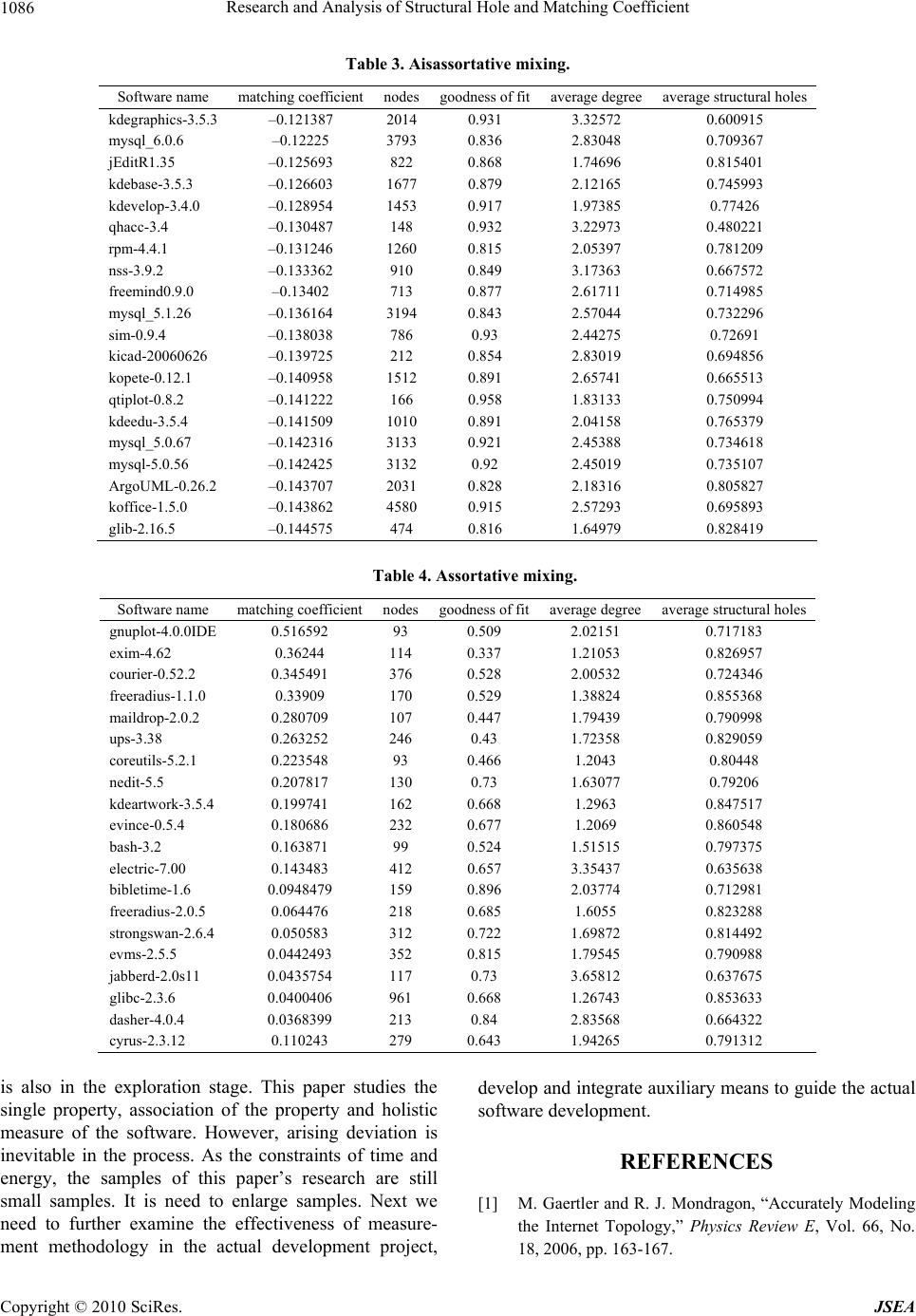

Research and Analysis of Structural Hole and Matching Coefficient

1086

Table 3. Aisassortative mixing.

Software name matching coefficientnodesgoodness of fitaverage degreeaverage structural holes

kdegraphics-3.5.3 –0.121387 20140.931 3.32572 0.600915

mysql_6.0.6 –0.12225 37930.836 2.83048 0.709367

jEditR1.35 –0.125693 822 0.868 1.74696 0.815401

kdebase-3.5.3 –0.126603 16770.879 2.12165 0.745993

kdevelop-3.4.0 –0.128954 14530.917 1.97385 0.77426

qhacc-3.4 –0.130487 148 0.932 3.22973 0.480221

rpm-4.4.1 –0.131246 12600.815 2.05397 0.781209

nss-3.9.2 –0.133362 910 0.849 3.17363 0.667572

freemind0.9.0 –0.13402 713 0.877 2.61711 0.714985

mysql_5.1.26 –0.136164 31940.843 2.57044 0.732296

sim-0.9.4 –0.138038 786 0.93 2.44275 0.72691

kicad-20060626 –0.139725 212 0.854 2.83019 0.694856

kopete-0.12.1 –0.140958 15120.891 2.65741 0.665513

qtiplot-0.8.2 –0.141222 166 0.958 1.83133 0.750994

kdeedu-3.5.4 –0.141509 10100.891 2.04158 0.765379

mysql_5.0.67 –0.142316 31330.921 2.45388 0.734618

mysql-5.0.56 –0.142425 31320.92 2.45019 0.735107

ArgoUML-0.26.2 –0.143707 20310.828 2.18316 0.805827

koffice-1.5.0 –0.143862 45800.915 2.57293 0.695893

glib-2.16.5 –0.144575 474 0.816 1.64979 0.828419

Table 4. Assortative mixing.

Software name matching coefficientnodesgoodness of fitaverage degreeaverage structural holes

gnuplot-4.0.0IDE 0.516592 93 0.509 2.02151 0.717183

exim-4.62 0.36244 114 0.337 1.21053 0.826957

courier-0.52.2 0.345491 376 0.528 2.00532 0.724346

freeradius-1.1.0 0.33909 170 0.529 1.38824 0.855368

maildrop-2.0.2 0.280709 107 0.447 1.79439 0.790998

ups-3.38 0.263252 246 0.43 1.72358 0.829059

coreutils-5.2.1 0.223548 93 0.466 1.2043 0.80448

nedit-5.5 0.207817 130 0.73 1.63077 0.79206

kdeartwork-3.5.4 0.199741 162 0.668 1.2963 0.847517

evince-0.5.4 0.180686 232 0.677 1.2069 0.860548

bash-3.2 0.163871 99 0.524 1.51515 0.797375

electric-7.00 0.143483 412 0.657 3.35437 0.635638

bibletime-1.6 0.0948479 159 0.896 2.03774 0.712981

freeradius-2.0.5 0.064476 218 0.685 1.6055 0.823288

strongswan-2.6.4 0.050583 312 0.722 1.69872 0.814492

evms-2.5.5 0.0442493 352 0.815 1.79545 0.790988

jabberd-2.0s11 0.0435754 117 0.73 3.65812 0.637675

glibc-2.3.6 0.0400406 961 0.668 1.26743 0.853633

dasher-4.0.4 0.0368399 213 0.84 2.83568 0.664322

cyrus-2.3.12 0.110243 279 0.643 1.94265 0.791312

is also in the exploration stage. This paper studies the

single property, association of the property and holistic

measure of the software. However, arising deviation is

inevitable in the process. As the constraints of time and

energy, the samples of this paper’s research are still

small samples. It is need to enlarge samples. Next we

need to further examine the effectiveness of measure-

ment methodology in the actual development project,

develop and integ rate auxiliary means to guide th e actual

software development.

REFERENCES

[1] M. Gaertler and R. J. Mondragon, “Accurately Modeling

the Internet Topology,” Physics Review E, Vol. 66, No.

18, 2006, pp. 163-167.

Research and Analysis of Structural Hole and Matching Coefficient 1087

[2] R. S. Burt, “Structural Holes: The Social Structure of

Competition,” Harvard University Press, 1995, PP. 35-38.

[3] S. Abdelwahed, N. Kandasamy and A. Gokhale, “High

Confidence Sofware for Cyber-Physical Systems,” Pro-

ceedings of the 2007 Workshop on Automating Service

Quality, Atlanta, 2007, PP. 1-3.

[4] Y. T. Ma, J. X. Chen and J. H. Wu, “Research on the

Phenomenon of Software Drift in Software Processes,”

Proceedings of 8th International Workshop on Principles

of Software Evolution, Lisbon, September 2005, pp.

195-198.

[5] M. Alshayeb and W. Li, “An Empirical Validation of

Object-Oriented Metrics in Two Different Iterative Soft-

ware Processes,” IEEE Transactions on Software Engi-

neering, Vol. 29, No. 11, November 2003, pp. 1043-

1049.

[6] L. C. Briand, S. Morasca and V. R. Basili, “Prop-

erty-Based Software Engineering Measurement,” IEEE

Transactions on Software Engineering, Vol. 22, No. 1,

January 1996, pp. 68-86.

[7] S. Furey, “Why We Should Use Function Points,” IEEE

Software, Vol. 14, No. 2, 1997, pp. 28-30.

[8] M. Arnold and P. Pedross, “Software Size Measurement

and Productivity Rating in a Large-Scale Software De-

velopment Department,” Proceedings of 20th Interna-

tional Conference on Software Engineering, Kyoto, 1998,

pp. 503-506.

[9] M. Bauer, “Analysing Software Systems by Using Com-

binations of Metrics,” Proceedings of ECOOP’99 Work-

shops, Lisbon, 1999, pp. 170-171.

[10] S. R. Chidamber and C. F. Kemerer, “A Metrics Suite for

Object-Oriented Design,” IEEE Transactions on Software

Engineering, Vol. 20, No. 6, June 1994, pp. 476-493.

[11] F. B. e Abreu, “The MOOD Metrics Set,” Proceedings of

ECOOP’95 Workshop on Metrics, Aarhus, 1995, pp.

150-152.

[12] N. E. Fenton and M. Neil, “Software Metrics: Successes,

Failures and New Directions,” Journal of Systems and

Software, Vol. 47, No. 2-3, July 1999, pp. 149-157.