Comparison of High Field Electron Transport in GaAs, InAs and In<sub>0.3</sub>Ga<sub>0.7</sub>As

doi:10.4236/jmp.2013.44A012

Paper Menu >>

Journal Menu >>

Journal of Modern Physics, 2013, 4, 121-126

http://dx.doi.org/10.4236/jmp.2013.44A012 Published Online April 2013 (http://www.scirp.org/journal/jmp)

Comparison of High Field Electron Transport in GaAs,

InAs and In0.3Ga0.7As

B. Bouazza, A. Guen-Bouazza, C. Sayah, N. E. Chabane-Sari

Unite de Recherches Matériaux et Energies Renouvelables, Faculté des Sciences de l’Ingénieur,

Université Abou-Bekr-Belkaïd de Tlemcen, Tlemcen, Algérie

Email: [email protected]

Received January 8, 2013; revised February 10, 2013; accepted February 25, 2013

which permits unrestricted use, distribution, and reproduction in any medium, provided the original work is properly cited.

ABSTRACT

An ensemble Monte Carlo simulation is used to compare high field electron transport in bulk GaAs, InAs and

In0.3Ga0.7As. In particular, velocity overshoot and electron transit times are examined. We find the steady state velocity

of the electrons is the most important factor determining transit time over distances longer then 0.2 μm. Over shorter

distances velocity overshoot effects in InAs and In0.3Ga0.7 As at high fields are comparable to those in GaAs. We esti-

mate the minimum transit time across a 1 μm InAs sample to be about 4.2 ps. Similar calculations for In0.3Ga0.7As yield

6 ps (for GaAs yield 10 ps). Calculations are made using a nonparabolic effective mass energy band model, Monte

Carlo simulation that includes all of the major scattering mechanisms. The band parameters used in the simulation are

extracted from optimized pseudopotential band calculations to ensure excellent agreement with experimental informa-

tion and ab initio band models.

Keywords: Monte Carlo Method; Semiconductor Devices; Velocity Overshoot; Electron Transport

1. Introduction

The Ensemble Monte Carlo technique has been used now

for over 30 years as a numerical method to simulate

nonequilibrium transport in semiconductor materials and

devices, and has been the subject of numerous books and

reviews. In application to transport problems, a random

walk is generated to simulate the stochastic motion of

particles subject to collision processes in some medium.

This process of random walk generation may be used to

evaluate integral equations and is connected to the gen-

eral random sampling technique used in the valuation of

multi-dimensional integrals. The basic technique is to

simulate the free particle motion (referred to as the free

flight) terminated by instantaneous random scattering

events. The Monte Carlo algorithm consists of generating

random free flight times for each particle, choosing the

type of scattering occurring at the end of the free flight,

changing the final energy and momentum of the particle

after scattering, and then repeating the procedure for the

next free flight. Sampling the particle motion at various

times throughout the simulation allows for the statistical

estimation of physically interesting quantities such as the

single particle distribution function, the average drift

velocity in the presence of an applied electric field, the

average energy of the particles, etc. By simulating an

ensemble of particles, representative of the physical sys-

tem of interest, the non-stationary time-dependent evolu-

tion of the electron and hole distributions under the in-

fluence of a time-dependent driving force may be simu-

lated. The particle-based picture, in which the particle

motion is decomposed into free flights terminated by

instantaneous collisions, is basically the same picture

underlying the derivation of the semi-classical BTE. In

fact, it may be shown that the one-particle distribution

function obtained from the random walk Monte Carlo

technique satisfies the BTE for a homogeneous system in

the long-time limit [1].

The purpose of this work is to compare, using Mont

Carlo simulation, the potentialities of n-type GaAs, InAs

and In0.3Ga0.7As. We first analyse, in Section 1, we ex-

plain how to apply our band structure model to Monte

Carlo simulation. In Section 2 we present to describe in

the detail our calculation of high field transport proper-

ties of n-type GaAs, InAs and In0.3Ga0.7As by Monte

Carlo method. We shall also compare our results with

other theoretical and experimental data insofar as it is

possible highlight the accuracy of the simulation results.

B. BOUAZZA ET AL.

122

1.1. Free Flight Generation

In the Monte Carlo method, the dynamics of particle mo-

tion is assumed to consist of free flights terminated by

instantaneous scattering events, which change the mo-

mentum and energy of the particle. To simulate this

process, the probability density







pt t



is required, in

which is the joint probability that a particle will

arrive at time t without scattering after the previous colli-

sion at t = 0, and then suffer a collision in a time interval

around time . The probability of scattering in the

time interval around t may be written as







kt t











,

where











is the scattering rate of an electron or

hole of wave vector . The scattering rate,













,

represents the sum of the contributions from each indi-

vidual scattering mechanism, which are usually calcu-

lated using perturbation theory, as described later. The

implicit dependence of















on time reflects the

change in due to acceleration by internal and external

fields [2-4]. For electrons subject to time independent

electric and magnetic fields, the time evolution of

between collisions as

 

0kt keEv B t







 (1)

where the electric field, is the electron velocity,

and



is the magnetic flux density. In terms of the

scattering rate,











tkt t





, the probability that a particle

has not suffered a collision after a time t is given by

exp













tt



k tt





.

Thus, the probability of scattering in the time interval

after a free flight of time may be written as the

joint probability

 

exp

Ptt kt









 













 (2)

Random flight times may be generated according to

the probability density



pt above using, for example,

the pseudo-random number generator implicit on most

modern computers, which generate uniformly distributed

random numbers in the range [0,1]. Using a direct

method, random flight times sampled from







tprr







may

be generated according to



rpt





 (3)

where r is a uniformly distributed random number and



is the desired free flight time. Integrating (3) with





ktt

















rktt





given by (2) above yields

1expr



 

 (4)

Since 1 − r is statistically the same as r, (4) may be

simplified to











(5)



Equation (5) is the fundamental equation used to gen-

erate the random free flight time after each scattering

event, resulting in a random walk process related to the

underlying particle distribution function. If there is no

external driving field leading to a change of between

scattering events, the time dependence vanishes, and the

integral is trivially evaluated. In the general case where

this simplification is not possible, it is expedient to in-

troduce the so called self-scattering method [1-3,5,6], in

which we introduce a fictitious scattering mechanism

whose scattering rate always adjusts itself in such a way

that the total (self-scattering plus real scattering) rate is a

constant in time





0Self





 

 (6)

where self



is the self-scattering rate. The self-scatter-

ing mechanism itself is defined such that the final state

before and after scattering is identical. Hence, it has no

effect on the free flight trajectory of a particle when se-

lected as the terminating scattering mechanism, yet re-

sults in the simplification of (5) such that the free flight is

given by



1ln

tr (7)

The constant total rate (including self-scattering) 0



is chosen a priori so that it is larger than the maximum

scattering encountered during the simulation interval. In

the simplest case, a single value is chosen at the begin-

ning of the entire simulation (constant gamma method),

checking to ensure that the real rate never exceeds this

value during the simulation. Other schemes may be cho-

sen that are more computationally efficient, and which

modify the choice of 0



at fixed time increments.

1.2. Selection of Scattering Rate

When the electrons are accelerated and the scattering

time is chosen, scattering must then occur at the end of

the scattering time period. The method used for this is the

rejection technique. This technique chooses the scattering

using the relative probabilities of the individual events.

To start we construct a scattering table and normalize all

scattering probabilities to the maximum scattering value,

which was found in the above section for the self scat-

tering [4]. Once the entire table is constructed, it can be

used throughout the entire simulation without need for

recompilation. The selection of the scattering now be-

comes a two-part step. As the table has already been

B. BOUAZZA ET AL. 123

normalized to one, we may use a uniform random num-

ber to select the scattering rate. The reason why this

works is simple. The choice of scattering is random, but

is also governed by the relative strength of certain scat-

tering rates in connection with others that exist in the

system. The random numbers take care of choosing the

scattering rate, and the relative strength of each scattering

rate to the total in the table controls the frequency of cer-

tain events over others.

1.3. Scattering Angle and Final State

For elastic scattering, the scattering is isotropic. There-

fore, all final states in the energy-conserving sphere have

the same probability of occupation after scattering. The

final angle is independent of the initial state , and the

angles of are proportional to

ksin





 

2π

cos

. Realiz-

ing that the azimuthal angle varies between 0 and , a

direct technique can be employed to obtain [2,4,7,8]:



 and 4

2πr



 (8)

1.4. Mean Velocity and Energy Calculation

When the electric field is applied in the x direction, the

average drift velocity and the average electron energy are

given for each valley, respectively, by [9],



vvt



















(10)

where











 (11)



114







 



 (12)

and



222

iyizi

kkkk



 (13)

where





vt and





i represent the electron drift

velocity and the electron energy at the end of each time

step, while



and

i are the wave vector com-

ponents in

y and direction for each electron, re-

spectively.

2. Simulation and Results

In each simulation, twenty thousand electrons are ini-

tially distributed in the sample according to an equilib-

rium Maxwellian distribution at 300 K. A variety of field

strengths are simulated to determine the effect on the

transient behavior of the electron ensemble. The simula-

tion steps the electric field from zero to full intensity at

the beginning of the run







, after which the velocity

of the electrons is averaged at 10fs intervals. The average

traveled as a function of time is found by integrating the

drift velocity. Our Monte Carlo program is based on a

three isotropic and non parabolic valley model. The pa-

rameters for valleys are estimated from recent band

structure calculations. The scattering mechanisms in-

cluded in the simulations are polar optical phonon,

acoustic phonons, piezoelectric, intervalley scattering,

ionized impurities and alloy scattering. Values for the

various coupling constants which determine many of the

scattering rates are the same as those used in Reference

[7]. The donor concentration is set to 1.107/cm3.

Figure 1 shows electron velocity versus distance for

GaAs, InAs and In0.3Ga0.7As. Previous Monte Carlo

studies of velocity overshoot in GaAs have performed

and are in agreement with the present results. We find the

fields which produce the highest steady state velocities (2

kv/cm in InAs and 5kv/cm in In0.3Ga0.7As) are similar to

the results using the full band Monte Carlo simulation.

Furthermore, in all three materials overshoot only occurs

at field strengths larger than the peak steady state veloc-

ity field and one sees that the higher amplitude of veloc-

ity overshoot, the lower its distance (or duration). These

observations are tentatively explained in the following

manner. First of all, we have checked that, as long as all

electrons remain in the



valley, the velocity increases.

Thus, the maximum velocity is reached when the “most

rapid” electrons have gained enough energy to transfer to

L valley. These electrons are “lucky electrons”, which

have suffered no, or very few, or very inefficient scatter-

ing events. Therefore, the time needed to reach the

maximum velocity is mainly determined quasiballistic

motion and is sensitive to the scattering rates. On the

contrary, the final static velocity is obtained when the

whole electron distribution has reached its new equilib-

rium situation. This process is completed when even

“unlucky” widely scattered, electrons have gained

enough energy to transfer.

Figure 2 shows the electron transit time as a function

of distance traveled. The field strengths transit time oc-

curs when the steady state velocity is the highest. Using

the relation





12πfT



 where





is the transit

time at 1 μm, we estimate the corresponding cutoff fre-

quencies for GaAs to 29 GHz. Values as high as 20 GHz

chosen minimize the electron transit time at 1 μm. In

GaAs, InAs and In0.3Ga0.7As the minimum have been

measured in modern GaAs modulation doped field

effect transistors, not far from the upper limit predicted

from the transit time alone.

1 μm

In Figure 3 we show the transit time as a function of

distance in the overshoot regime. In this figure the ap-

plied fields were chosen to minimize the transit time

B. BOUAZZA ET AL.

124

0.0 1.0x10-7 2.0x10-7 3.0x10-7 4.0x10-7

1x105

2x105

3x105

4x105

5x105

5.0x10-7

0.0 2.0x10-7 4.0x 10-7 6.0x10-7 8.0x10-7 1.0x

0.0

2.0x105

4.0x105

6.0x105

8.0x105

1.0x106

10-6 1.2x10-6

0.0 2.0x10-7 4.0x10-7

0.0

2.0x105

4.0x105

6.0x105

8.0x105

6.0x10-7

Figure 1. Electron velocity as function of distance in each of the materials simulated.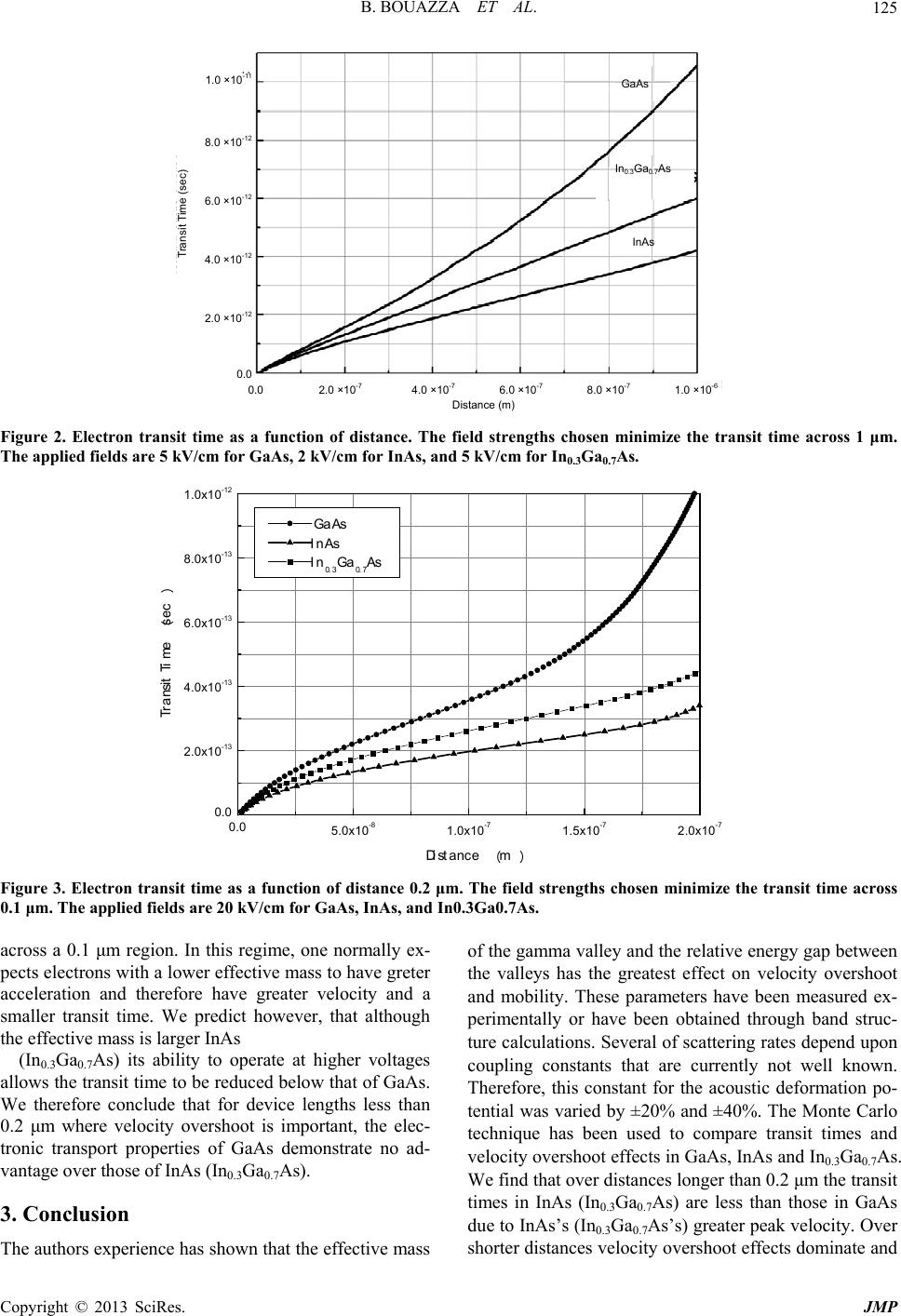

B. BOUAZZA ET AL. 125

1.0 ×10-

8.0 ×10-12

6.0 ×10-12

4.0 ×10-12

2.0 ×10-12

0.0

Transit Time (sec)

0.0 2.0 ×10-7 4.0 ×10

-7 6.0 ×10

-7 8.0 ×10

-7 1.0 ×10

-6

Distance (m)

GaAs

In0.3Ga0.7As

InAs

Figure 2. Electron transit time as a function of distance. The field strengths chosen minimize the transit time across 1 μm.

The applied fields are 5 kV/cm for GaAs, 2 kV/cm for InAs, and 5 kV/cm for In0.3Ga0.7As.

0.0 5.0x10-8 1.0x10-7 1.5x10-7

0.0

2.0x10-13

4.0x10-13

6.0x10-13

8.0x10-13

1.0x10-12

2.0x10-7

Figure 3. Electron transit time as a function of distance 0.2 μm. The field strengths chosen minimize the transit time across

0.1 μm. The applied fields are 20 kV/cm for GaAs, InAs, and In0.3Ga0.7As.

across a 0.1 μm region. In this regime, one normally ex-

pects electrons with a lower effective mass to have greter

acceleration and therefore have greater velocity and a

smaller transit time. We predict however, that although

the effective mass is larger InAs

(In0.3Ga0.7As) its ability to operate at higher voltages

allows the transit time to be reduced below that of GaAs.

We therefore conclude that for device lengths less than

0.2 μm where velocity overshoot is important, the elec-

tronic transport properties of GaAs demonstrate no ad-

vantage over those of InAs (In0.3Ga0.7As).

3. Conclusion

The authors experience has shown that the effective mass

of the gamma valley and the relative energy gap between

the valleys has the greatest effect on velocity overshoot

and mobility. These parameters have been measured ex-

perimentally or have been obtained through band struc-

ture calculations. Several of scattering rates depend upon

coupling constants that are currently not well known.

Therefore, this constant for the acoustic deformation po-

tential was varied by ±20% and ±40%. The Monte Carlo

technique has been used to compare transit times and

velocity overshoot effects in GaAs, InAs and In0.3Ga0.7As.

We find that over distances longer than 0.2 μm the transit

times in InAs (In0.3Ga0.7As) are less than those in GaAs

due to InAs’s (In0.3Ga0.7As’s) greater peak velocity. Over

shorter distances velocity overshoot effects dominate and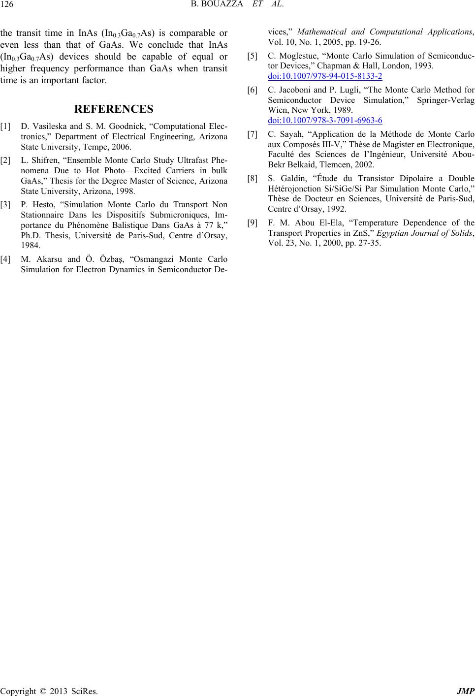

B. BOUAZZA ET AL.

126

the transit time in InAs (In0.3Ga0.7As) is comparable or

even less than that of GaAs. We conclude that InAs

(In0.3Ga0.7As) devices should be capable of equal or

higher frequency performance than GaAs when transit

time is an important factor.

REFERENCES

[1] D. Vasileska and S. M. Goodnick, “Computational Elec-

tronics,” Department of Electrical Engineering, Arizona

State University, Tempe, 2006.

[2] L. Shifren, “Ensemble Monte Carlo Study Ultrafast Phe-

nomena Due to Hot Photo—Excited Carriers in bulk

GaAs,” Thesis for the Degree Master of Science, Arizona

State University, Arizona, 1998.

[3] P. Hesto, “Simulation Monte Carlo du Transport Non

Stationnaire Dans les Dispositifs Submicroniques, Im-

portance du Phénomène Balistique Dans GaAs à 77 k,”

Ph.D. Thesis, Université de Paris-Sud, Centre d’Orsay,

1984.

[4] M. Akarsu and Ö. Özbaş, “Osmangazi Monte Carlo

Simulation for Electron Dynamics in Semiconductor De-

vices,” Mathematical and Computational Applications,

Vol. 10, No. 1, 2005, pp. 19-26.

[5] C. Moglestue, “Monte Carlo Simulation of Semiconduc-

tor Devices,” Chapman & Hall, London, 1993.

doi:10.1007/978-94-015-8133-2

[6] C. Jacoboni and P. Lugli, “The Monte Carlo Method for

Semiconductor Device Simulation,” Springer-Verlag

Wien, New York, 1989.

doi:10.1007/978-3-7091-6963-6

[7] C. Sayah, “Application de la Méthode de Monte Carlo

aux Composés III-V,” Thèse de Magister en Electronique,

Faculté des Sciences de l’Ingénieur, Université Abou-

Bekr Belkaid, Tlemcen, 2002.

[8] S. Galdin, “Étude du Transistor Dipolaire a Double

Hétérojonction Si/SiGe/Si Par Simulation Monte Carlo,”

Thèse de Docteur en Sciences, Université de Paris-Sud,

Centre d’Orsay, 1992.

[9] F. M. Abou El-Ela, “Temperature Dependence of the

Transport Properties in ZnS,” Egyptian Journal of Solids,

Vol. 23, No. 1, 2000, pp. 27-35.