Response of the Plankton to a Fresh Water Pulse in a Fresh Water Deprived, Permanently Open South African Estuary

doi:10.4236/jwarp.2013.54040

Paper Menu >>

Journal Menu >>

Journal of Water Resource and Protection, 2013, 5, 405-413

http://dx.doi.org/10.4236/jwarp.2013.54040 Published Online April 2013 (http://www.scirp.org/journal/jwarp)

Response of the Plankton to a Fresh Water Pulse in a Fresh

Water Deprived, Permanently Open South African Estuary

Pierre William Froneman1*, Paul Denzi Vorwerk2

1Coastal Research Group, Department of Zoology and Entomology, Rhodes University, Grahamstown, South Africa

2South African Environmental Observation Network (SAEON) Elwandle Node, Grahamstown, South Africa

Email: *[email protected]

Received January 17, 2013; revised February 28, 2013; accepted March 10, 2013

Commons Attribution License, which permits unrestricted use, distribution, and reproduction in any medium, provided the original

work is properly cited.

ABSTRACT

This study assessed the influence of a freshwater pulse on selected physico-chemical and biological variables in a per-

manently open freshwater deprived southern African estuary. In the absence of the freshwater pulse a reverse gradient

in salinity was evident with hypersaline (salinity > 40) conditions prevailing in the upper reaches of the estuary. Total

chlorophyll-a (chl-a) concentration during this period ranged from 0.25 to 0.60 µg·l−1. The mean total zooplankton

abundance and biomass in the absence of freshwater during the daytime was 666 ind·m−3 (SD ± 196) and 12.4

mg·dwt·m−3 (SD ± 3.3), respectively. During the night time the mean total zooplankton abundance was 3121 ind·m−3

(SD ± 1203) and the biomass 21.8 mg·dwt·m−3 (SD ± 196). The total zooplankton abundance during the dry season was

numerically dominated by the copepod nauplii and the calanoid copepod, Pseudodiaptomus hessei, which contributed

up to 76% of the total zooplankton counts. The freshwater pulse was associated with the establishment of a horizontal

gradient in salinity along the length of the estuary and a significant increase in the total chl-a concentration (range from

0.74 to 11.75 µg·l−1) and zooplankton biomass (range from 23.7 to 76.6 mg·dwt·m−3) (p < 0.05 in both cases). Addition-

ally, there was a marked increase in the total zooplankton abundances and biomass within the estuary. A distinct shift in

the zooplankton community composition was evident with the copepod, Acartia longipatella numerically dominating

the zooplankton counts.

Keywords: Estuary Zooplankton Community; Freshwater Inflow

1. Introduction

Increased population growth coupled with industrializa-

tion has coincided with a decrease in the magnitude of

freshwater flowing into southern African estuaries. The

influence of the reduced freshwater inflow on the biology

of southern African estuaries is now well documented [1,

2]. Reduced freshwater inflow into estuaries has been

linked to a decrease in the phytoplankton size composi-

tion and daily production rates largely because freshwa-

ter inflow represents the primary source of nutrients nec-

essary to sustain the growth of the phytoplankton, par-

ticularly diatoms [1,3,4]. Among the heterotrophic com-

ponents of the estuarine food web, the alteration in the

riverine inflow into estuaries has been linked to changes

in the recruitment, biomass and species composition and

distribution of both inverstebrates and vertebrates within

these systems [2,5,6]. The formation of horizontal salin-

ity gradients in estuaries is also associated with spatial

patterns in the plankton biomass (so-called river-estuary

interface (REI) zone [7] Finally, freshwater inflow into

estuaries has been linked an increased diversity of niches

and food sources available to animals in these systems

[8-10].

The Kariega Estuary on the south-east coast of South

Africa is regarded as a fresh water deprived system and

has been reported as having hypersaline conditions in the

upper reaches in various studies since 1991 [11-13]. The

hypersaline conditions in the upper reaches of the estuary

can be attributed to reduced freshwater inflow as a result

of small catchment area (≈680 km2), the presence of sev-

eral impoundments along the Kariega River and high

evaporative losses, particularly during the summer months

[12,13]. Localised flooding occurred during September

2006 along the south-east coast of South Africa, resulting

in a horizontal salinity gradient being recorded within the

system for the first time since 1991. The biological res-

*Corresponding author.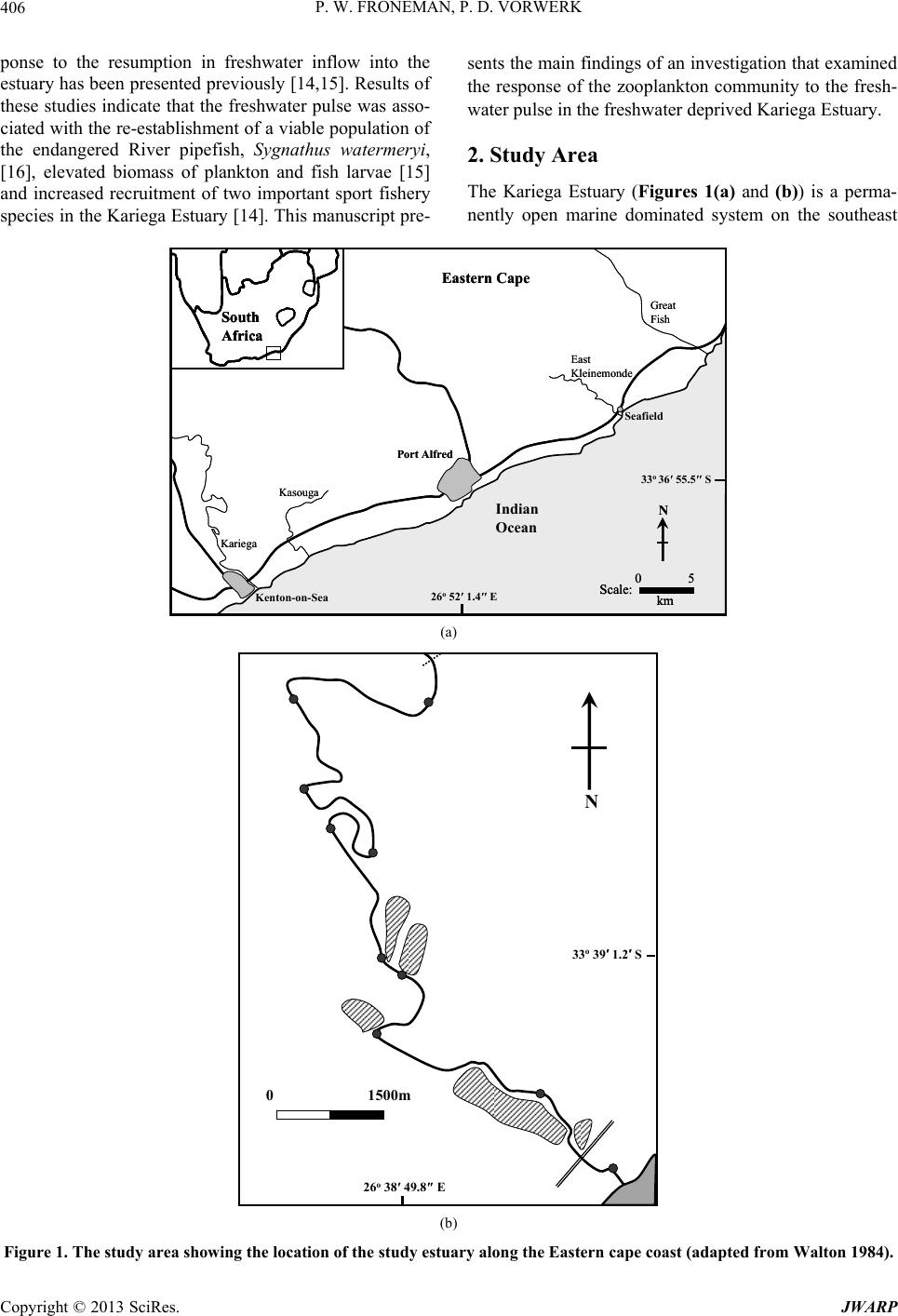

P. W. FRONEMAN, P. D. VORWERK

406

ponse to the resumption in freshwater inflow into the

estuary has been presented previously [14,15]. Results of

these studies indicate that the freshwater pulse was asso-

ciated with the re-establishment of a viable population of

the endangered River pipefish, Sygnathus watermeryi,

[16], elevated biomass of plankton and fish larvae [15]

and increased recruitment of two important sport fishery

species in the Kariega Estuary [14]. This manuscript pre-

sents the main findings of an investigation that examined

the response of the zooplankton community to the fresh-

water pulse in the freshwater deprived Kariega Estuary.

2. Study Area

The Kariega Estuary (Figures 1(a) and (b)) is a perma-

nently open marine dominated system on the southeast

Port Alfred

Seafield

Eastern Cape

Kenton-on-Sea

Indian

Ocean

South

Africa

East

Kleinemonde

Great

Fish

0 5

Kasouga

Kariega

Scale:

36′55.5″S

52′1.4″E

Port Alfred

Seafield

Eastern Cape

Kenton-on-Sea

Indian

Ocean

South

Africa

South

Africa

East

Kleinemonde

Great

Fish

0 5

Kasouga

Kariega

0 5

Scale:Scale:Scale: kmkm

36′55.5″S

52′1.4″E

(a)

33o39′1.2′S

26o38′49.8″E

0 1500m

33o39′1.2′S

26o38′49.8″E

0 1500m

33o39′1.2′S

26o38′49.8″E

0 1500m

(b)

Figure 1. The study area showing the location of the study estuary along the Eastern cape coast (adapted from Walton 1984).

P. W. FRONEMAN, P. D. VORWERK 407

coast of South Africa (33˚40'46.6"S; 26˚40'57.9"E) [14]

The estuary is approximately 18 km long, has a depth

range of 2.5 m to 3.5 m and varies in width between 40

m and 100 m [7,13] The estuary is predominantly marine

with hypersaline conditions being recorded in the upper

reaches since 1991 [3,11,13]. The dominance of the ma-

rine environment within the system is indicated by the

106:1 ratio of tidal prism volume to river flow volume

[17]. The middle reaches of the estuary are characterised

by extensive salt marshes comprising the high marsh

plants Sarcocornia perennis, Chenolea diffusa and Spar-

tina maritima. The marine dominance of the system has

also contributed to the eelgrass, Zostera capensis, ex-

tending its distribution along the length of the estuary

[7,13].

3. Materials and Methods

Sampling of the zooplankton and related physico-che-

mical variables was conducted during November 2005

and November 2006. The November 2005 sampling re-

presents the flow rates at present (low flow rates, design-

nated dry season) within the system, while the November

2006 sampling represents a wet season for the Kariega

Estuary. Sampling was conducted at 10 stations along the

length of the Kariega Estuary during daylight and night

time during low tide.

3.1. Physico-Chemical Variables

Temperature and salinity (practical salinity units) at each

station were measured using a Horiba U10 water sampler

at both the surface and bottom of the water column with-

in the estuary.

3.2. Chlorophyll-a (chl-a)

Chlorophyll-a concentrations were determined for sur-

face and bottom waters for each station by collecting 200

ml water sample using an 8 L Niskin bottle. These sam-

ples were vacuum filtered (<5 cm Hg) through GF/F fil-

ters which were subsequently extracted in 90% acetone

for 24 hr in the dark at −20˚C. The total chlorophyll-a

concentrations were then determined using a 10AU-Tur-

ner flourometer before and after acidification according

to the method of Holm-Hansen and Riemann [18].

3.3. Zooplankton

Zooplankton at each station was collected during three

replicate surface tows (depth ≈ 0.5 m) conducted during

the day and night using a WP-2 Net (50 cm diameter,

100 μm mesh) fitted with a General Oceanics flow meter

to allow for volumetric standardisation of the samples.

All samples collected were stored in 10% buffered for-

malin for later identification in the laboratory. For each

replicate sample the zooplankton dry biomass was de-

termined by filtering a 1/2 to 1/32 sub-sample, obtained

using a Folsom plankton splitter, through a pre-weighed

GF/F filter and then oven drying at 60˚C for a period of

24 hr. The dry biomass was calculated as the difference

between the filter weight and the combined dry weight.

All zooplankton were counted to allow for density esti-

mates which were then averaged across the three repli-

cate samples. Abundance and biomass values were ex-

pressed as ind·m−3 and mg·dwt·m−3, respectively.

3.4. Numerical Analyses

The average community abundance data for each station

was entered into the PRIMER (Plymouth Routines in

Multivariate Ecological Research version 5.2.4 software

package for comparison between the stations [19]. The

data was transformed (log(x + 1)) to minimise the effect

of less abundant species and input into a group-averaged

Bray-Curtis Similarity analysis from which a cluster dia-

gram was generated. The SIMPER routine was then em-

ployed to identify which species were contributing to the

differences between the groupings identified with the nu-

merical analysis [19].

3.5. Statistical Analyses

To test for differences between wet and dry seasons for

chlorophyll concentrations, zooplankton biomass and

zooplankton densities, a Lilliefors test for normality was

used prior to inputting the data into an ANOVA. These

statistical tests were run in the STATISTICA for Win-

dows package [20].

4. Results

4.1. Flow Data

The monthly flow volumes in the four months preceding

the dry season sampling (from June to September) in

2005, never exceeded 0.026 × 106 m

3 with a maximum

occurring in June 2005 (Figure 2). The monthly flow

volumes increased from 0.012 × 106 m3 in June 2006 to

4.45 × 106 m3 and 2.9 × 106 m3 in August and September,

respectively (Figure 2) (Department of Water Affairs

and Forestry Flow Data).

4.2. Physico-Chemical Variables

The temperature profiles recorded during both the wet

and dry seasons were similar, with a temperature gradient

evident from the mouth to the head of the system (Figure

3). Temperatures during the dry season (November 2005)

ranged from 19.3˚C near the mouth to 23.4˚C at the head

of the estuary, while during the wet season (November

2006) the lower reach temperatures were 17.4˚C with a

maximum of 24˚C at the head. The recorded salinity

P. W. FRONEMAN, P. D. VORWERK

408

Month

JuneJulyAugust September

Monthly Flow Volume (million m3)

0.00

0.01

0.02

0.03

2.50

3.00

3.50

4.00

4.50 2005

2006

Figure 2. The monthly flow volume (million m3) in the months preceding the sampling during 2005 and 2006 (drawn from

Department of Water Affairs and Forestry Flow Data).

Depth (m)

0.0

0.5

1.0

1.5

Distance from Mouth (km)

2 4 6 810121416

Depth (m)

0.0

0.5

1.0

1.5

(b)

(a)

Figure 3. Contour plots of the temperature (˚C) in the Kariega Estuary during the dry season, November 2005 (a); and the

wet season, November 2006 (b).

demonstrated a reverse salinity gradient during the dry

season, with a minimum salinity of 35 near the mouth of

the estuary and a maximum of 36.5 near the head of the

system (Figure 4). Conversely, during the wet season, a

normal salinity gradient was evident, with salinities of 34

recorded at the mouth and 4.7 at the head of the estuary

(Figure 4). A salt wedge was also evident in the upper

reaches of the system during the wet season, with salini-

ties on the bottom less than 12.

4.3. Chlorophyll-a

The total chlorophyll-a concentration during the dry sea-

son was relatively uniform along the length of the estuary,

and ranged from 0.25 μg·L−1 to 0.61 μg·L−1 (Figure 5).

No apparent horizontal or vertical patterns were evident

in the total chlorophyll-a concentration during the dry

season. During the wet season, the total chlorophyll-a

concentration was significantly higher (p < 0.001; F =

34.08), ranging from 0.74 μg·L−1 to a maximum of 11.75

μg·L−1. During the wet season the maximum chlorophyll-

a concentration occurred in the mixing zone between oli-

gohaline and polyhaline conditions approximately 14 km

from the mouth (Figures 4 and 5).

4.4. Zooplankton

Daytime dry season densities of zooplankton ranged

from 432 ind·m−3 to 936 ind·m−3, while during the wet

season total zooplankton densities varied between 76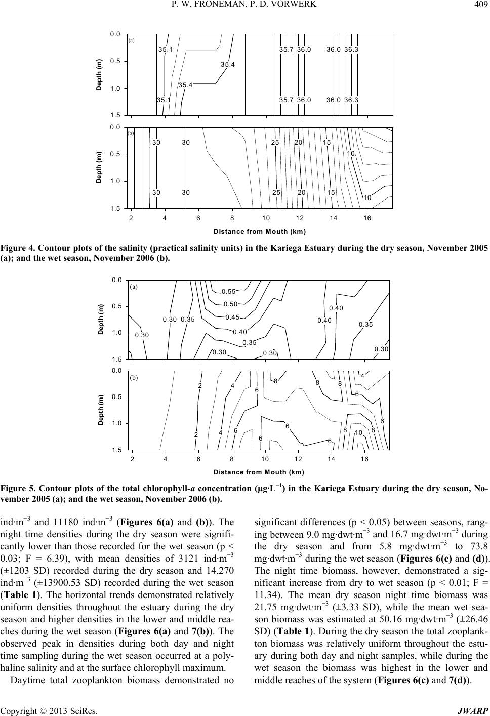

P. W. FRONEMAN, P. D. VORWERK 409

35.4

35.1

36.0

35.7

36.0

36.3

Depth (m)

0.0

0.5

1.0

1.5

Distance from Mouth (km)

246810 12 14 16

Depth (m)

0.0

0.5

1.0

1.5

(a)

(b)

Figure 4. Contour plots of the salinity (practical salinity units) in the Kariega Estuary during the dry season, November 2005

(a); and the wet season, November 2006 (b).

0.30

0.35

0.30

0.35

0.30

0.55

0.50

0.45

0.40

0.30

0.40

0.35

0.30

Depth (m)

0.0

0.5

1.0

1.5

Distance from Mouth (km)

246810121416

Depth (m)

0.0

0.5

1.0

1.5

(a)

(b)

Figure 5. Contour plots of the total chlorophyll-a concentration (μg·L−1) in the Kariega Estuary during the dry season, No-

vember 2005 (a); and the wet season, November 2006 (b).

ind·m−3 and 11180 ind·m−3 (Figures 6(a) and (b)). The

night time densities during the dry season were signifi-

cantly lower than those recorded for the wet season (p <

0.03; F = 6.39), with mean densities of 3121 ind·m−3

(±1203 SD) recorded during the dry season and 14,270

ind·m−3 (±13900.53 SD) recorded during the wet season

(Table 1). The horizontal trends demonstrated relatively

uniform densities throughout the estuary during the dry

season and higher densities in the lower and middle rea-

ches during the wet season (Figures 6(a) and 7(b)). The

observed peak in densities during both day and night

time sampling during the wet season occurred at a poly-

haline salinity and at the surface chlorophyll maximum.

Daytime total zooplankton biomass demonstrated no

significant differences (p < 0.05) between seasons, rang-

ing between 9.0 mg·dwt·m−3 and 16.7 mg·dwt·m−3 during

the dry season and from 5.8 mg·dwt·m−3 to 73.8

mg·dwt·m−3 during the wet season (Figures 6(c) and (d)).

The night time biomass, however, demonstrated a sig-

nificant increase from dry to wet season (p < 0.01; F =

11.34). The mean dry season night time biomass was

21.75 mg·dwt·m−3 (±3.33 SD), while the mean wet sea-

son biomass was estimated at 50.16 mg·dwt·m−3 (±26.46

SD) (Table 1). During the dry season the total zooplank-

ton biomass was relatively uniform throughout the estu-

ary during both day and night samples, while during the

wet season the biomass was highest in the lower and

middle reaches of the system (Figures 6(c) and 7(d)).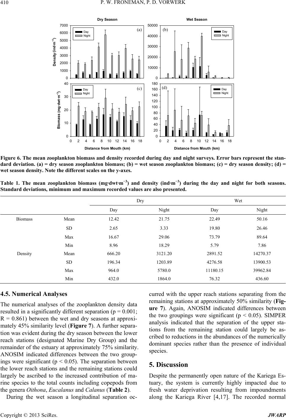

P. W. FRONEMAN, P. D. VORWERK

410

Dry Season

Distance from Mouth (km)

024681012141618

Biomass (mg dwt m-3)

Day

Night

Wet Seaso

Distance from M

outh (km)

0246810

Density (ind.m-3)

1000

2000

3000

4000

5000

6000

7000

Day

Night

10000

20000

30000

40000

50000

Day

Night

12141618

100

120

140

160

180

Day

Night

(a) (b)

(ind·m

−3

)

(mg·dwt·m

−3

)

Figure 6. The mean zooplankton biomass and density recorded during day and night surveys. Error bars represent the stan-

dard deviation. (a) = dry season zooplankton biomass; (b) = wet season zooplankton biomass; (c) = dry season density; (d) =

wet season density. Note the different scales on the y-axes.

Table 1. The mean zooplankton biomass (mg·dwt·m−3) and density (ind·m−3) during the day and night for both seasons.

Standard deviations, minimum and maximum recorded values are also presented.

Dry Wet

Day Night Day Night

Biomass Mean 12.42 21.75 22.49 50.16

SD 2.65 3.33 19.80 26.46

Max 16.67 29.06 73.79 89.64

Min 8.96 18.29 5.79 7.86

Density Mean 666.20 3121.20 2891.52 14270.37

SD 196.34 1203.89 4276.58 13900.53

Max 964.0 5780.0 11180.15 39962.84

Min 432.0 1864.0 76.32 436.60

4.5. Numerical Analyses

The numerical analyses of the zooplankton density data

resulted in a significantly different separation (p = 0.001;

R = 0.861) between the wet and dry seasons at approxi-

mately 45% similarity level (Figure 7). A further separa-

tion was evident during the dry season between the lower

reach stations (designated Marine Dry Group) and the

remainder of the estuary at approximately 75% similarity.

ANOSIM indicated differences between the two group-

ings were significant (p < 0.05). The separation between

the lower reach stations and the remaining stations could

largely be ascribed to the increased contribution of ma-

rine species to the total counts including copepods from

the genera Oithona, Eucalanus and Calanus (Table 2).

During the wet season a longitudinal separation oc-

curred with the upper reach stations separating from the

remaining stations at approximately 50% similarity (Fig-

ure 7). Again, ANOSIM indicated differences between

the two groupings were significant (p < 0.05). SIMPER

analysis indicated that the separation of the upper sta-

tions from the remaining station could largely be as-

cribed to reductions in the abundances of the numerically

dominant species rather than the presence of individual

species.

5. Discussion

Despite the permanently open nature of the Kariega Es-

tuary, the system is currently highly impacted due to

fresh water deprivation resulting from impoundments

along the Kariega River [4,17]. The recorded normal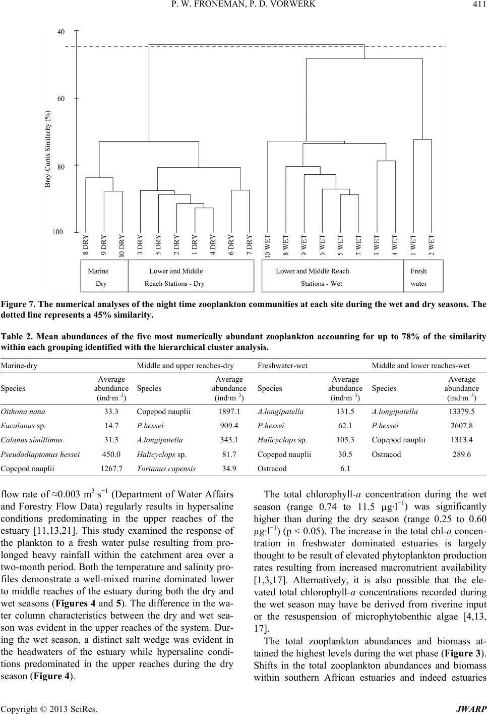

P. W. FRONEMAN, P. D. VORWERK 411

Figure 7. The numerical analyses of the night time zooplankton communities at each site during the wet and dry seasons. The

dotted line represents a 45% similarity.

Table 2. Mean abundances of the five most numerically abundant zooplankton accounting for up to 78% of the similarity

within each grouping identified with the hierarchical cluster analysis.

Marine-dry Middle and upper reaches-dry Freshwater-wet Middle and lower reaches-wet

Species

Average

abundance

(ind·m−3)

Species

Average

abundance

(ind·m−3)

Species

Average

abundance

(ind·m−3)

Species

Average

abundance

(ind·m−3)

Oithona nana 33.3 Copepod nauplii 1897.1 A.longipatella 131.5 A.longipatella 13379.5

Eucalanus sp. 14.7 P.hessei 909.4 P.hessei 62.1 P.hessei 2607.8

Calanus simillimus 31.3 A.longipatella 343.1 Halicyclops sp. 105.3 Copepod nauplii 1313.4

Pseudodiapto mus h essei 450.0 Halicyclops sp. 81.7 Copepod nauplii30.5 Ostracod 289.6

Copepod nauplii 1267.7 Tortanus capensis34.9 Ostracod 6.1

flow rate of ≈0.003 m3·s−1 (Department of Water Affairs

and Forestry Flow Data) regularly results in hypersaline

conditions predominating in the upper reaches of the

estuary [11,13,21]. This study examined the response of

the plankton to a fresh water pulse resulting from pro-

longed heavy rainfall within the catchment area over a

two-month period. Both the temperature and salinity pro-

files demonstrate a well-mixed marine dominated lower

to middle reaches of the estuary during both the dry and

wet seasons (Figures 4 and 5). The difference in the wa-

ter column characteristics between the dry and wet sea-

son was evident in the upper reaches of the system. Dur-

ing the wet season, a distinct salt wedge was evident in

the headwaters of the estuary while hypersaline condi-

tions predominated in the upper reaches during the dry

season (Figure 4).

The total chlorophyll-a concentration during the wet

season (range 0.74 to 11.5 µg·l−1) was significantly

higher than during the dry season (range 0.25 to 0.60

µg·l−1) (p < 0.05). The increase in the total chl-a concen-

tration in freshwater dominated estuaries is largely

thought to be result of elevated phytoplankton production

rates resulting from increased macronutrient availability

[1,3,17]. Alternatively, it is also possible that the ele-

vated total chlorophyll-a concentrations recorded during

the wet season may have be derived from riverine input

or the resuspension of microphytobenthic algae [4,13,

17].

The total zooplankton abundances and biomass at-

tained the highest levels during the wet phase (Figure 3).

Shifts in the total zooplankton abundances and biomass

within southern African estuaries and indeed estuaries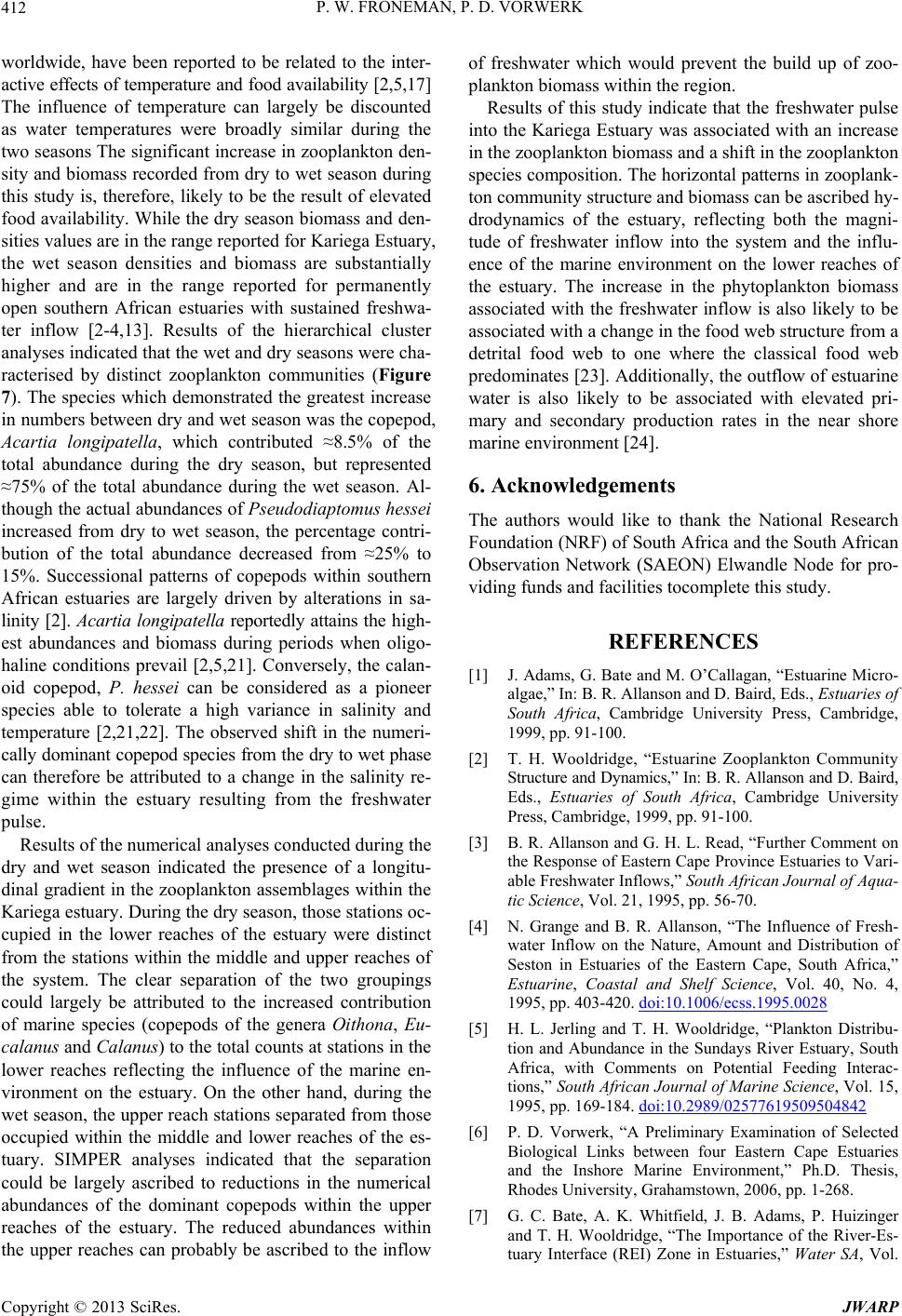

P. W. FRONEMAN, P. D. VORWERK

412

worldwide, have been reported to be related to the inter-

active effects of temperature and food availability [2,5,17]

The influence of temperature can largely be discounted

as water temperatures were broadly similar during the

two seasons The significant increase in zooplankton den-

sity and biomass recorded from dry to wet season during

this study is, therefore, likely to be the result of elevated

food availability. While the dry season biomass and den-

sities values are in the range reported for Kariega Estuary,

the wet season densities and biomass are substantially

higher and are in the range reported for permanently

open southern African estuaries with sustained freshwa-

ter inflow [2-4,13]. Results of the hierarchical cluster

analyses indicated that the wet and dry seasons were cha-

racterised by distinct zooplankton communities (Figure

7). The species which demonstrated the greatest increase

in numbers between dry and wet season was the copepod,

Acartia longipatella, which contributed ≈8.5% of the

total abundance during the dry season, but represented

≈75% of the total abundance during the wet season. Al-

though the actual abundances of Pseudodiaptomus hessei

increased from dry to wet season, the percentage contri-

bution of the total abundance decreased from ≈25% to

15%. Successional patterns of copepods within southern

African estuaries are largely driven by alterations in sa-

linity [2]. Acartia longipatella reportedly attains the high-

est abundances and biomass during periods when oligo-

haline conditions prevail [2,5,21]. Conversely, the calan-

oid copepod, P. hessei can be considered as a pioneer

species able to tolerate a high variance in salinity and

temperature [2,21,22]. The observed shift in the numeri-

cally dominant copepod species from the dry to wet phase

can therefore be attributed to a change in the salinity re-

gime within the estuary resulting from the freshwater

pulse.

Results of the numerical analyses conducted during the

dry and wet season indicated the presence of a longitu-

dinal gradient in the zooplankton assemblages within the

Kariega estuary. During the dry season, those stations oc-

cupied in the lower reaches of the estuary were distinct

from the stations within the middle and upper reaches of

the system. The clear separation of the two groupings

could largely be attributed to the increased contribution

of marine species (copepods of the genera Oithona, Eu-

calanus and Calanus) to the total counts at stations in the

lower reaches reflecting the influence of the marine en-

vironment on the estuary. On the other hand, during the

wet season, the upper reach stations separated from those

occupied within the middle and lower reaches of the es-

tuary. SIMPER analyses indicated that the separation

could be largely ascribed to reductions in the numerical

abundances of the dominant copepods within the upper

reaches of the estuary. The reduced abundances within

the upper reaches can probably be ascribed to the inflow

of freshwater which would prevent the build up of zoo-

plankton biomass within the region.

Results of this study indicate that the freshwater pulse

into the Kariega Estuary was associated with an increase

in the zooplankton biomass and a shift in the zooplankton

species composition. The horizontal patterns in zooplank-

ton community structure and biomass can be ascribed hy-

drodynamics of the estuary, reflecting both the magni-

tude of freshwater inflow into the system and the influ-

ence of the marine environment on the lower reaches of

the estuary. The increase in the phytoplankton biomass

associated with the freshwater inflow is also likely to be

associated with a change in the food web structure from a

detrital food web to one where the classical food web

predominates [23]. Additionally, the outflow of estuarine

water is also likely to be associated with elevated pri-

mary and secondary production rates in the near shore

marine environment [24].

6. Acknowledgements

The authors would like to thank the National Research

Foundation (NRF) of South Africa and the South African

Observation Network (SAEON) Elwandle Node for pro-

viding funds and facilities tocomplete this study.

REFERENCES

[1] J. Adams, G. Bate and M. O’Callagan, “Estuarine Micro-

algae,” In: B. R. Allanson and D. Baird, Eds., Estuaries of

South Africa, Cambridge University Press, Cambridge,

1999, pp. 91-100.

[2] T. H. Wooldridge, “Estuarine Zooplankton Community

Structure and Dynamics,” In: B. R. Allanson and D. Baird,

Eds., Estuaries of South Africa, Cambridge University

Press, Cambridge, 1999, pp. 91-100.

[3] B. R. Allanson and G. H. L. Read, “Further Comment on

the Response of Eastern Cape Province Estuaries to Vari-

able Freshwater Inflows,” South African Journal of Aqua-

tic Science, Vol. 21, 1995, pp. 56-70.

[4] N. Grange and B. R. Allanson, “The Influence of Fresh-

water Inflow on the Nature, Amount and Distribution of

Seston in Estuaries of the Eastern Cape, South Africa,”

Estuarine, Coastal and Shelf Science, Vol. 40, No. 4,

1995, pp. 403-420. doi:10.1006/ecss.1995.0028

[5] H. L. Jerling and T. H. Wooldridge, “Plankton Distribu-

tion and Abundance in the Sundays River Estuary, South

Africa, with Comments on Potential Feeding Interac-

tions,” South African Journal of Marine Science, Vol. 15,

1995, pp. 169-184. doi:10.2989/02577619509504842

[6] P. D. Vorwerk, “A Preliminary Examination of Selected

Biological Links between four Eastern Cape Estuaries

and the Inshore Marine Environment,” Ph.D. Thesis,

Rhodes University, Grahamstown, 2006, pp. 1-268.

[7] G. C. Bate, A. K. Whitfield, J. B. Adams, P. Huizinger

and T. H. Wooldridge, “The Importance of the River-Es-

tuary Interface (REI) Zone in Estuaries,” Water SA, Vol.

P. W. FRONEMAN, P. D. VORWERK

413

28, No. 3, 2002, pp. 271-279.

[8] A. K. Whitfield and M. N. Bruton, “Some Biological Im-

plications of Reduced Fresh Water Inflow into Eastern

Cape Estuaries: A Preliminary Assessment,” South Afri-

can Journal of Science, Vol. 85, 1989, pp. 691-694.

[9] L. D. Ter, E. R. Morshuizen and A. K. Whitfield, “The

Distribution of Littoral Fish Associated with Eelgrass

Zostera capensis in the Kariega Estuary, a Southern Af-

rican System with a Reversed Salinity Gradient,” South

African Journal of Marine Science, Vol. 14, 1994, pp. 95-

105. doi:10.2989/025776194784287049

[10] A. K. Whitfield and T. H. Wooldridge, “Changes in

Freshwater Supplies to Southern African Estuaries: Some

Theoretical and Practical Considerations,” In: K. R. Dyer

and R. J. Orth, Eds., Changes in Fluxes in Estuaries: Im-

plications from Science to Management, Olsen & Olsen,

Fredensborg, 1994, pp. 41-50.

[11] L. D. Ter Morshuizen, A. K. Whitfield and A. W. Pater-

son, “Influence of Freshwater Flow Regime on Fish As-

semblages in the Great Fish River and Estuary,” South

African Journal of Aquatic Science, Vol. 22, 1996, pp.

52-61.

[12] A. K. Whitfield and A. W. Paterson, “Distribution Pat-

terns of Fishes in a Freshwater Deprived Eastern Cape

Estuary, with Particular Emphasis on the Geographical

Headwater Region,” Water SA, Vol. 29, No. 1, 2003, pp.

61-67.

[13] E. E. Heyns and P. W. Froneman,“Spatial and Temporal

Patterns in the Hyperbenthic Community Structure in Sou-

thern African Permanently Open Estuary,” Estuarine,

Coastal and Shelf Science, Vol. 88, 2010, pp. 105-115.

[14] P. D. Vorwerk, A. W. Paterson, P. W. Froneman and A.

K. Whitfield, “Increased Abundance of Two Important

Sport Fishery Species Following Renewed River Flow

into a Freshwater Deprived South African Estuary,” Fish-

eries Management and Ecology, Vol. 16, No. 5, 2009, pp.

420-423. doi:10.1111/j.1365-2400.2009.00687.x

[15] P. D. Vorwerk, P. W. Froneman, A. W. Paterson, N. A.

Strydom and A. K. Whitfield, “Biological Responses to a

Resumption in River Flow in a Freshwater Deprived,

Permanently Open Southern African Estuary,” Water SA,

Vol. 34, No. 5, 2008, pp. 597-604.

[16] P. D. Vorwerk, P. W. Froneman and A. W. Paterson, “Re-

vival of the Critically Endangered River Pipefish, Syn-

gnathus watermeyeri, in Eastern Cape Estuaries,” South

African Journal of Science, Vol. 103, 2007, pp. 193-195.

[17] N. Grange, A. K. Whitfield, C. J. De Villiers and B. R.

Allanson, “The Response of Two South African East

Coast Estuaries to Altered River Flow Regimes,” Aquatic

Conservation: Marine and Freshwater Ecosystems, Vol.

10, No. 3, 2000, pp. 155-177.

doi:10.1002/1099-0755(200005/06)10:3<155::AID-AQC

406>3.0.CO;2-Z

[18] O. Holm-Hansen and B. Riemann, “Chlorophyll-a Deter-

mination: Improvements in Methodology,” Oikos, Vol. 30,

No. 3, 1978, pp. 438-447. doi:10.2307/3543338

[19] K. R. Clarke and R. M. Warwick, “Change in Marine

Communities: An Approach to Statistical Analysis and

Interpretation,” Plymouth Marine Laboratory, Plymouth,

1994.

[20] Statsoft Inc., “Statistica, Data Analysis Software System,”

Version 7, 2004

[21] N. A. Strydom, A. K. Whitfield, A. W. Paterson, N. A.

Strydom, A. K. Whitfield and A. W. Paterson, “Influence

of Altered Freshwater Flow Regimes on Abundance of

Larval and Juvenile Gilchristella aestuaria (Pisces: Clu-

peidae) in the Upper Reaches of Two South African Es-

tuaries,” Marine and Freshwater Research, Vol. 69, 2002,

pp. 178-189.

[22] P. W. Froneman, “Response of the Plankton to Three Dif-

ferent Hydrological Phases of the Temporarily Open/

Closed Kasouga Estuary, South Africa,” Estuarine, Coas-

tal and Shelf Science, Vol. 55, 2002, pp. 535-546.

doi:10.1006/ecss.2001.0921

[23] A. W. Paterson and A. K. Whitfield, “A Stable Carbon

Isotope Study of the Food-Web in a Freshwater-Deprived

South African Estuary, with Particular Emphasis on the

Ichthyofauna,” Estuarine, Coastal and Shelf Science, Vol.

45, 1997, pp. 705-715. doi:10.1006/ecss.1997.0243

[24] P. D. Vorwerk and P. W. Froneman, “The Importance of

Estuarine Derived Carbon for the Near Shore Marine En-

vironment: Studies on Contrasting Southern African Es-

tuaries,” African Journal of Aquatic Science, Vol. 34, 2009,

pp. 67-77. doi:10.2989/AJAS.2009.34.2.4.891