Predicting Soil Corrosivity along a Pipeline Route in the Niger Delta Basin Using Geoelectrical Method: Implications for Corrosion Control

doi:10.4236/eng.2013.53034

Paper Menu >>

Journal Menu >>

Engineering, 2013, 5, 237-244

http://dx.doi.org/10.4236/eng.2013.53034 Published Online March 2013 (http://www.scirp.org/journal/eng)

Predicting Soil Corrosivity along a Pipeline Route in the

Niger Delta Basin Using Geoelectrical Method:

Implications for Corrosion Control

Kenneth S. Okiongbo*, Godwin Ogobiri

Department of Geology & Physics, Niger Delta University, Bayelsa State, Nigeria

Email: *[email protected]

Received November 29, 2012; revised February 18, 2013; accepted February 25, 2013

ABSTRACT

The corrosivity of the top three metres of the soil along a pipeline route was determined using soil electrical resistivity

for the emplacement of a conduit intended to serve as a gas pipeline. Fifty-six Schlumberger vertical electrical sound-

ings (VES) were carried using a maximum current electrode separation ranging between 24 - 100 m at 2.0 km interval.

The data were interpreted using a 1D inversion technique software (1X1D, Interpex, USA). Model resistivity values

were classified in terms of the degree of corrosivity. Generally, the sub-soil condition along the pipeline route is

non-aggressive but being slightly or moderately aggressive in certain areas due to local conditions prevailing at the

measuring stations. Based on the corrosivity along the pipeline route, appropriate cathodic protection methods are pre-

scribed.

Keywords: Soil Corrosivity; Geoelectrical; Pipeline; Groundbed; Niger Delta

1. Introduction

The Niger Delta Basin is one of the prolific crude oil

provinces in the world and as such there is an extensive

network of pipelines. Pipelines play an extremely impor-

tant role through-out the world as a means of transporting

gases and liquids over long distances from their sources

of production to distribution terminals. A buried operat-

ing pipeline is unobtrusive and is rarely known except at

valves, pumping, compressor stations or terminals, hence

it is a preferred means of transportation of gases and liq-

uids. A vast majority of underground pipelines is made

of carbon steel, and these steels have inadequate alloy

additions to be considered corrosion resistant and un-

dergo a variety of corrosion failure modes/mechanisms in

underground environments, including general corrosion,

pitting corrosion, and stress-corrosion cracking (SCC) [1].

Given the implications of pipeline failures, and the role

that external corrosion plays in these failures, it is ap-

parent that prediction of corrosion and thus proper corro-

sion control can have a major impact on the safety, envi-

ronmental preservation and the economics of pipeline

operation.

In this instance, a circular conduit of approximately

110 km in length was planned to be built from Obirikom

(Rivers State) to Oben (Edo State) in the Niger Delta

Basin, Nigeria. The conduit would serve as a gas pipeline.

The engineers involved in the project considered that the

conduit would be trenched. Soil corrosion in this case

was anticipated in regards to the pipeline which is ex-

pected to be buried within the top three metres of the soil.

Ruptured pipelines due to corrosion failure are ubiqui-

tous in the Niger Delta, resulting in crude oil spills with

devastating ecological consequences. The control and

effective minimization of corrosion are possible by the

proper understanding of the material characteristics and

performance as well as the conditions of the environment

in which the material will reside. This enhances the de-

sign life of steel components and structures in contact

with the soil. Aside, it saves money, improves safety and

protects the environment. A key requirement to prevent

corrosion and thus ensure a satisfactory performance of a

piping system is the design and installation of an effec-

tive cathodic protection system. The cathodic protection

(CP) system is a proven, highly effective and elegant

method of corrosion control. CP can be either galvanic or

impressed current cathodic protection system, depending

on whether the soil resistivity is low or high. Soil corro-

sivity is not a measureable parameter. Therefore, in the

evaluation of soil corrossivity/aggressivity, a host of

critical parameters characteristic of the soil are usually

employed. These include soil kind, condition, water con-

tent, pH value, redox potentials, microbiological activity,

*Corresponding author.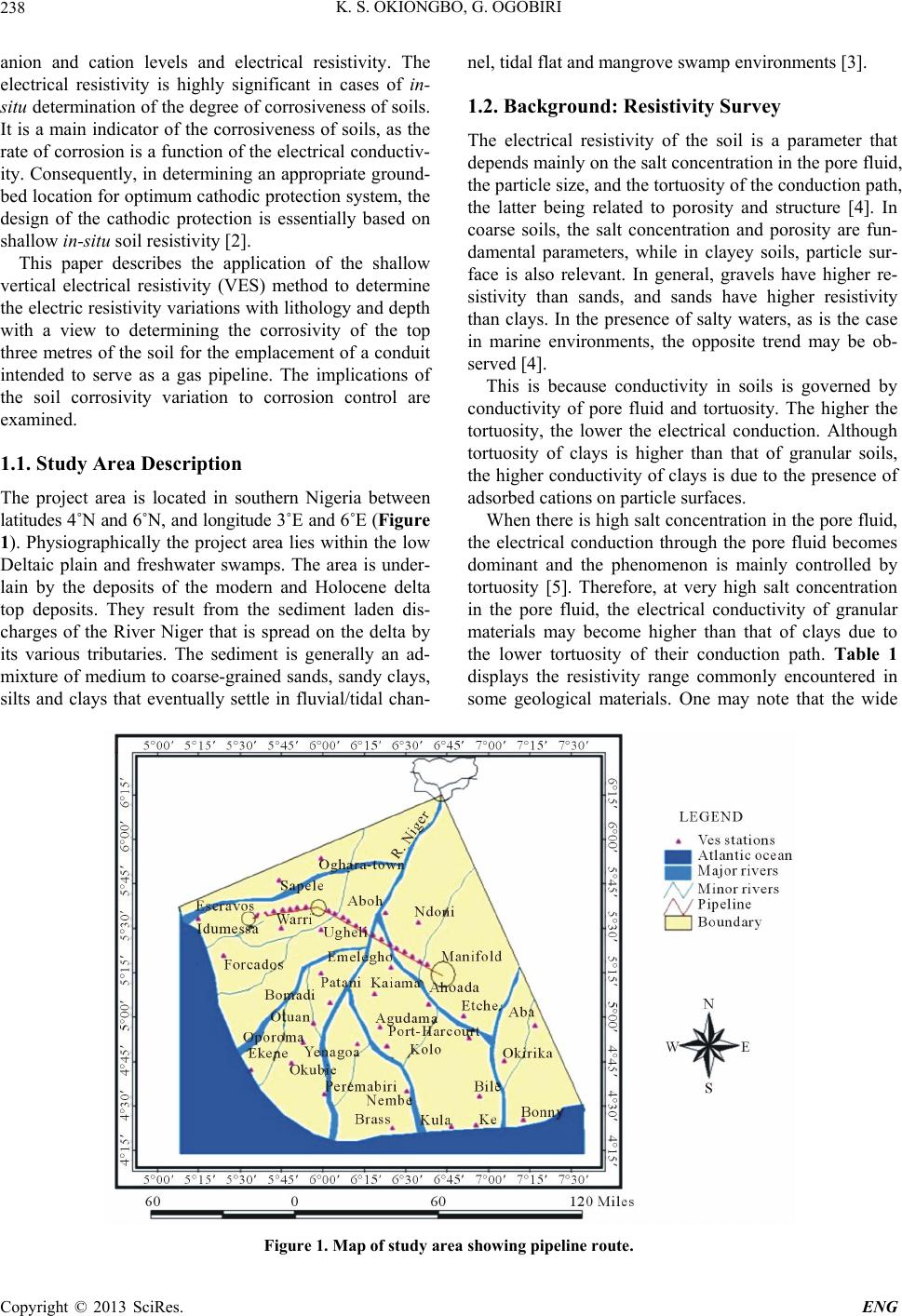

K. S. OKIONGBO, G. OGOBIRI

238

anion and cation levels and electrical resistivity. The

electrical resistivity is highly significant in cases of in-

situ determination of the degree of corrosiveness of soils.

It is a main indicator of the corrosiveness of soils, as the

rate of corrosion is a function of the electrical conductiv-

ity. Consequently, in determining an appropriate ground-

bed location for optimum cathodic protection system, the

design of the cathodic protection is essentially based on

shallow in-situ soil resistivity [2].

This paper describes the application of the shallow

vertical electrical resistivity (VES) method to determine

the electric resistivity variations with lithology and depth

with a view to determining the corrosivity of the top

three metres of the soil for the emplacement of a conduit

intended to serve as a gas pipeline. The implications of

the soil corrosivity variation to corrosion control are

examined.

1.1. Study Area Description

The project area is located in southern Nigeria between

latitudes 4˚N and 6˚N, and longitude 3˚E and 6˚E (Figure

1). Physiographically the project area lies within the low

Deltaic plain and freshwater swamps. The area is under-

lain by the deposits of the modern and Holocene delta

top deposits. They result from the sediment laden dis-

charges of the River Niger that is spread on the delta by

its various tributaries. The sediment is generally an ad-

mixture of medium to coarse-grained sands, sandy clays,

silts and clays that eventually settle in fluvial/tidal chan-

nel, tidal flat and mangrove swamp environments [3].

1.2. Background: Resistivity Survey

The electrical resistivity of the soil is a parameter that

depends mainly on the salt concentration in the pore fluid,

the particle size, and the tortuosity of the conduction path,

the latter being related to porosity and structure [4]. In

coarse soils, the salt concentration and porosity are fun-

damental parameters, while in clayey soils, particle sur-

face is also relevant. In general, gravels have higher re-

sistivity than sands, and sands have higher resistivity

than clays. In the presence of salty waters, as is the case

in marine environments, the opposite trend may be ob-

served [4].

This is because conductivity in soils is governed by

conductivity of pore fluid and tortuosity. The higher the

tortuosity, the lower the electrical conduction. Although

tortuosity of clays is higher than that of granular soils,

the higher conductivity of clays is due to the presence of

adsorbed cations on particle surfaces.

When there is high salt concentration in the pore fluid,

the electrical conduction through the pore fluid becomes

dominant and the phenomenon is mainly controlled by

tortuosity [5]. Therefore, at very high salt concentration

in the pore fluid, the electrical conductivity of granular

materials may become higher than that of clays due to

the lower tortuosity of their conduction path. Table 1

displays the resistivity range commonly encountered in

some geological materials. One may note that the wide

Figure 1. Map of study area showing pipeline route.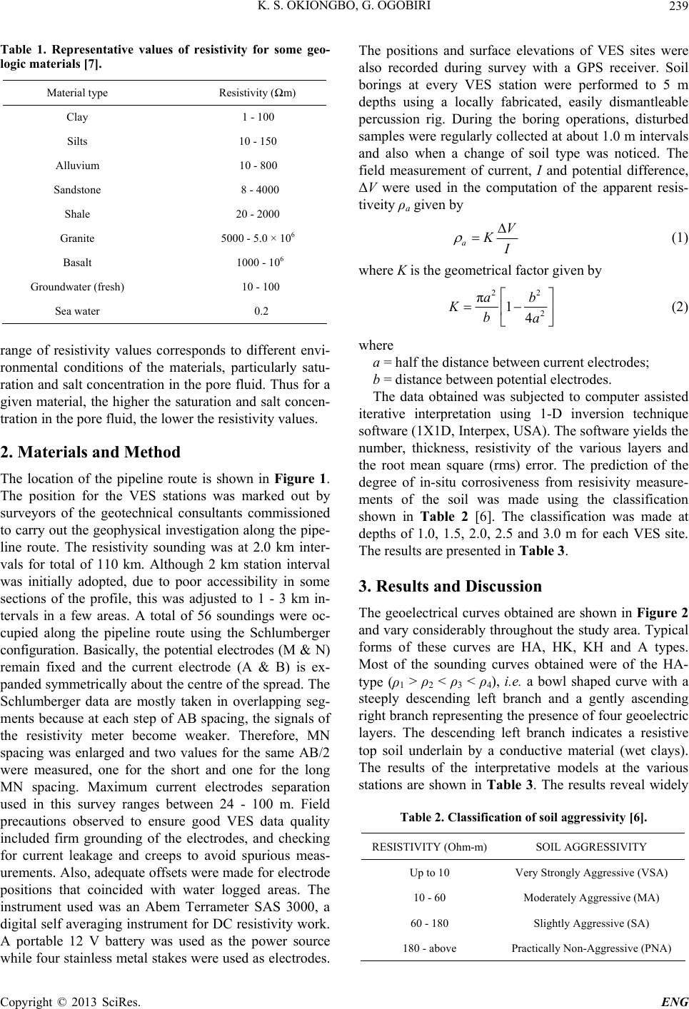

K. S. OKIONGBO, G. OGOBIRI 239

Table 1. Representative values of resistivity for some geo-

logic materials [7].

Material type Resistivity (m)

Clay 1 - 100

Silts 10 - 150

Alluvium 10 - 800

Sandstone 8 - 4000

Shale 20 - 2000

Granite 5000 - 5.0 × 106

Basalt 1000 - 106

Groundwater (fresh) 10 - 100

Sea water 0.2

range of resistivity values corresponds to different envi-

ronmental conditions of the materials, particularly satu-

ration and salt concentration in the pore fluid. Thus for a

given material, the higher the saturation and salt concen-

tration in the pore fluid, the lower the resistivity values.

2. Materials and Method

The location of the pipeline route is shown in Figure 1.

The position for the VES stations was marked out by

surveyors of the geotechnical consultants commissioned

to carry out the geophysical investigation along the pipe-

line route. The resistivity sounding was at 2.0 km inter-

vals for total of 110 km. Although 2 km station interval

was initially adopted, due to poor accessibility in some

sections of the profile, this was adjusted to 1 - 3 km in-

tervals in a few areas. A total of 56 soundings were oc-

cupied along the pipeline route using the Schlumberger

configuration. Basically, the potential electrodes (M & N)

remain fixed and the current electrode (A & B) is ex-

panded symmetrically about the centre of the spread. The

Schlumberger data are mostly taken in overlapping seg-

ments because at each step of AB spacing, the signals of

the resistivity meter become weaker. Therefore, MN

spacing was enlarged and two values for the same AB/2

were measured, one for the short and one for the long

MN spacing. Maximum current electrodes separation

used in this survey ranges between 24 - 100 m. Field

precautions observed to ensure good VES data quality

included firm grounding of the electrodes, and checking

for current leakage and creeps to avoid spurious meas-

urements. Also, adequate offsets were made for electrode

positions that coincided with water logged areas. The

instrument used was an Abem Terrameter SAS 3000, a

digital self averaging instrument for DC resistivity work.

A portable 12 V battery was used as the power source

while four stainless metal stakes were used as electrodes.

The positions and surface elevations of VES sites were

also recorded during survey with a GPS receiver. Soil

borings at every VES station were performed to 5 m

depths using a locally fabricated, easily dismantleable

percussion rig. During the boring operations, disturbed

samples were regularly collected at about 1.0 m intervals

and also when a change of soil type was noticed. The

field measurement of current, I and potential difference,

V were used in the computation of the apparent resis-

tiveity ρa given by





 (1)

where K is the geometrical factor given by

14

Kba













 (2)

where

a = half the distance between current electrodes;

b = distance between potential electrodes.

The data obtained was subjected to computer assisted

iterative interpretation using 1-D inversion technique

software (1X1D, Interpex, USA). The software yields the

number, thickness, resistivity of the various layers and

the root mean square (rms) error. The prediction of the

degree of in-situ corrosiveness from resisivity measure-

ments of the soil was made using the classification

shown in Table 2 [6]. The classification was made at

depths of 1.0, 1.5, 2.0, 2.5 and 3.0 m for each VES site.

The results are presented in Table 3.

3. Results and Discussion

The geoelectrical curves obtained are shown in Figure 2

and vary considerably throughout the study area. Typical

forms of these curves are HA, HK, KH and A types.

Most of the sounding curves obtained were of the HA-

type (ρ1 > ρ2 < ρ3 < ρ4), i.e. a bowl shaped curve with a

steeply descending left branch and a gently ascending

right branch representing the presence of four geoelectric

layers. The descending left branch indicates a resistive

top soil underlain by a conductive material (wet clays).

The results of the interpretative models at the various

stations are shown in Table 3. The results reveal widely

Table 2. Classification of soil aggressivity [6].

RESISTIVITY (Ohm-m)SOIL AGGRESSIVITY

Up to 10 Very Strongly Aggressive (VSA)

10 - 60 Moderately Aggressive (MA)

60 - 180 Slightly Aggressive (SA)

180 - above Practically Non-Aggressive (PNA)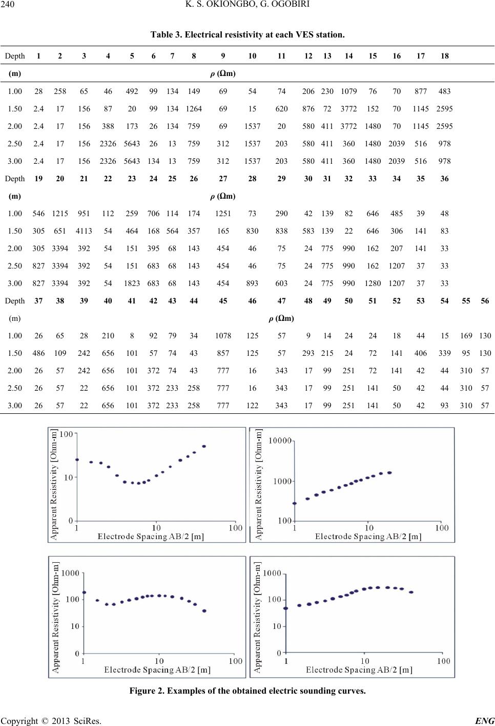

K. S. OKIONGBO, G. OGOBIRI

240

Table 3. Electrical resistivity at each VES station.

Depth 1 2 3 4 5 6 7 8 9 1011 12131415 16 17 18

(m) ρ (Ωm)

1.00 28 258 65 46 492 99 134 14969 5474 206230107976 70 877 483

1.50 2.4 17 156 87 20 99 134 126469 15620 876723772152 70 1145 2595

2.00 2.4 17 156 388 173 26 134 75969 153720 58041137721480 70 1145 2595

2.50 2.4 17 156 2326 5643 26 13 759312 1537203 5804113601480 2039 516 978

3.00 2.4 17 156 2326 5643 134 13 759312 1537203 5804113601480 2039 516 978

Depth 19 20 21 22 23 24 25 2627 2829 303132 33 34 35 36

(m) ρ (Ωm)

1.00 546 1215 951 112 259 706 114 1741251 73290 4213982646 485 39 48

1.50 305 651 4113 54 464 168 564 357165 830838 58313922646 306 141 83

2.00 305 3394 392 54 151 395 68 143454 4675 24775990162 207 141 33

2.50 827 3394 392 54 151 683 68 143454 4675 24775990162 1207 37 33

3.00 827 3394 392 54 1823 683 68 143454 893603 247759901280 1207 37 33

Depth 37 38 39 40 41 42 43 4445 4647 484950 51 52 53 545556

(m) ρ (Ωm)

1.00 26 65 28 210 8 92 79 341078 12557 91424 24 18 44 15169130

1.50 486 109 242 656 101 57 74 43857 12557 2932152472 141 406 33995130

2.00 26 57 242 656 101 372 74 43777 16343 179925172 141 42 4431057

2.50 26 57 22 656 101 372 233 258777 16343 1799251141 50 42 4431057

3.00 26 57 22 656 101 372 233 258777 122343 1799251141 50 42 9331057

Figure 2. Examples of the obtained electric sounding curves.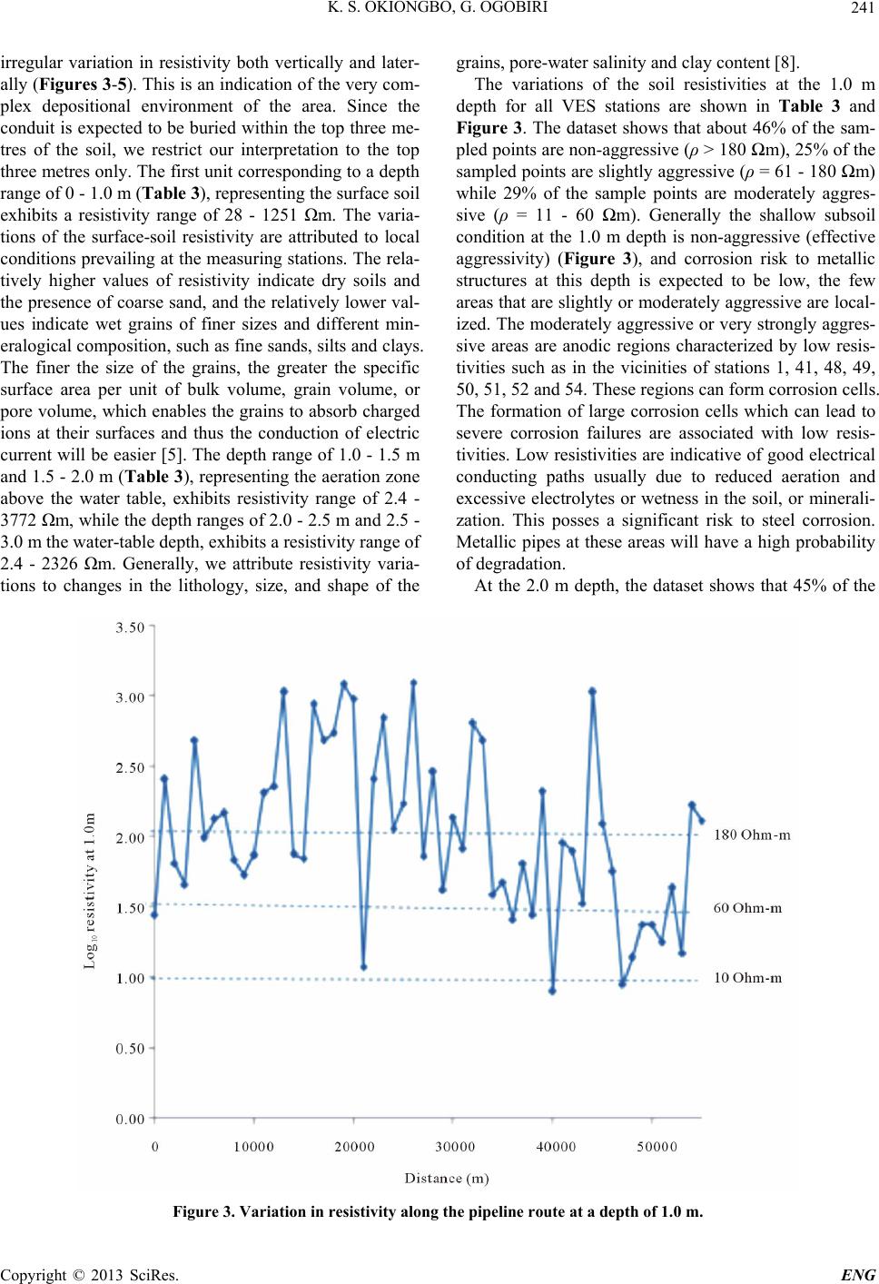

K. S. OKIONGBO, G. OGOBIRI 241

irregular variation in resistivity both vertically and later-

ally (Figures 3-5). This is an indication of the very com-

plex depositional environment of the area. Since the

conduit is expected to be buried within the top three me-

tres of the soil, we restrict our interpretation to the top

three metres only. The first unit corresponding to a depth

range of 0 - 1.0 m (Table 3), representing the surface soil

exhibits a resistivity range of 28 - 1251 m. The varia-

tions of the surface-soil resistivity are attributed to local

conditions prevailing at the measuring stations. The rela-

tively higher values of resistivity indicate dry soils and

the presence of coarse sand, and the relatively lower val-

ues indicate wet grains of finer sizes and different min-

eralogical composition, such as fine sands, silts and clays.

The finer the size of the grains, the greater the specific

surface area per unit of bulk volume, grain volume, or

pore volume, which enables the grains to absorb charged

ions at their surfaces and thus the conduction of electric

current will be easier [5]. The depth range of 1.0 - 1.5 m

and 1.5 - 2.0 m (Table 3), representing the aeration zone

above the water table, exhibits resistivity range of 2.4 -

3772 m, while the depth ranges of 2.0 - 2.5 m and 2.5 -

3.0 m the water-table depth, exhibits a resistivity range of

2.4 - 2326 m. Generally, we attribute resistivity varia-

tions to changes in the lithology, size, and shape of the

grains, pore-water salinity and clay content [8].

The variations of the soil resistivities at the 1.0 m

depth for all VES stations are shown in Table 3 and

Figure 3. The dataset shows that about 46% of the sam-

pled points are non-aggressive (ρ > 180 m), 25% of the

sampled points are slightly aggressive (ρ = 61 - 180 m)

while 29% of the sample points are moderately aggres-

sive (ρ = 11 - 60 m). Generally the shallow subsoil

condition at the 1.0 m depth is non-aggressive (effective

aggressivity) (Figure 3), and corrosion risk to metallic

structures at this depth is expected to be low, the few

areas that are slightly or moderately aggressive are local-

ized. The moderately aggressive or very strongly aggres-

sive areas are anodic regions characterized by low resis-

tivities such as in the vicinities of stations 1, 41, 48, 49,

50, 51, 52 and 54. These regions can form corrosion cells.

The formation of large corrosion cells which can lead to

severe corrosion failures are associated with low resis-

tivities. Low resistivities are indicative of good electrical

conducting paths usually due to reduced aeration and

excessive electrolytes or wetness in the soil, or minerali-

zation. This posses a significant risk to steel corrosion.

Metallic pipes at these areas will have a high probability

of degradation.

At the 2.0 m depth, the dataset shows that 45% of the

Figure 3. Variation in resistivity along the pipeline route at a depth of 1.0 m.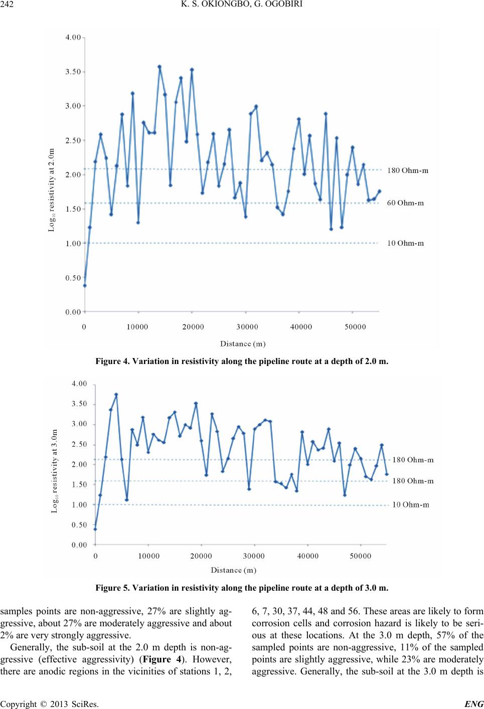

K. S. OKIONGBO, G. OGOBIRI

242

Figure 4. Variation in resistivity along the pipeline route at a depth of 2.0 m.

Figure 5. Variation in resistivity along the pipeline route at a depth of 3.0 m.

samples points are non-aggressive, 27% are slightly ag-

gressive, about 27% are moderately aggressive and about

2% are very strongly aggressive.

Generally, the sub-soil at the 2.0 m depth is non-ag-

gressive (effective aggressivity) (Figure 4). However,

there are anodic regions in the vicinities of stations 1, 2,

6, 7, 30, 37, 44, 48 and 56. These areas are likely to form

corrosion cells and corrosion hazard is likely to be seri-

ous at these locations. At the 3.0 m depth, 57% of the

sampled points are non-aggressive, 11% of the sampled

points are slightly aggressive, while 23% are moderately

aggressive. Generally, the sub-soil at the 3.0 m depth is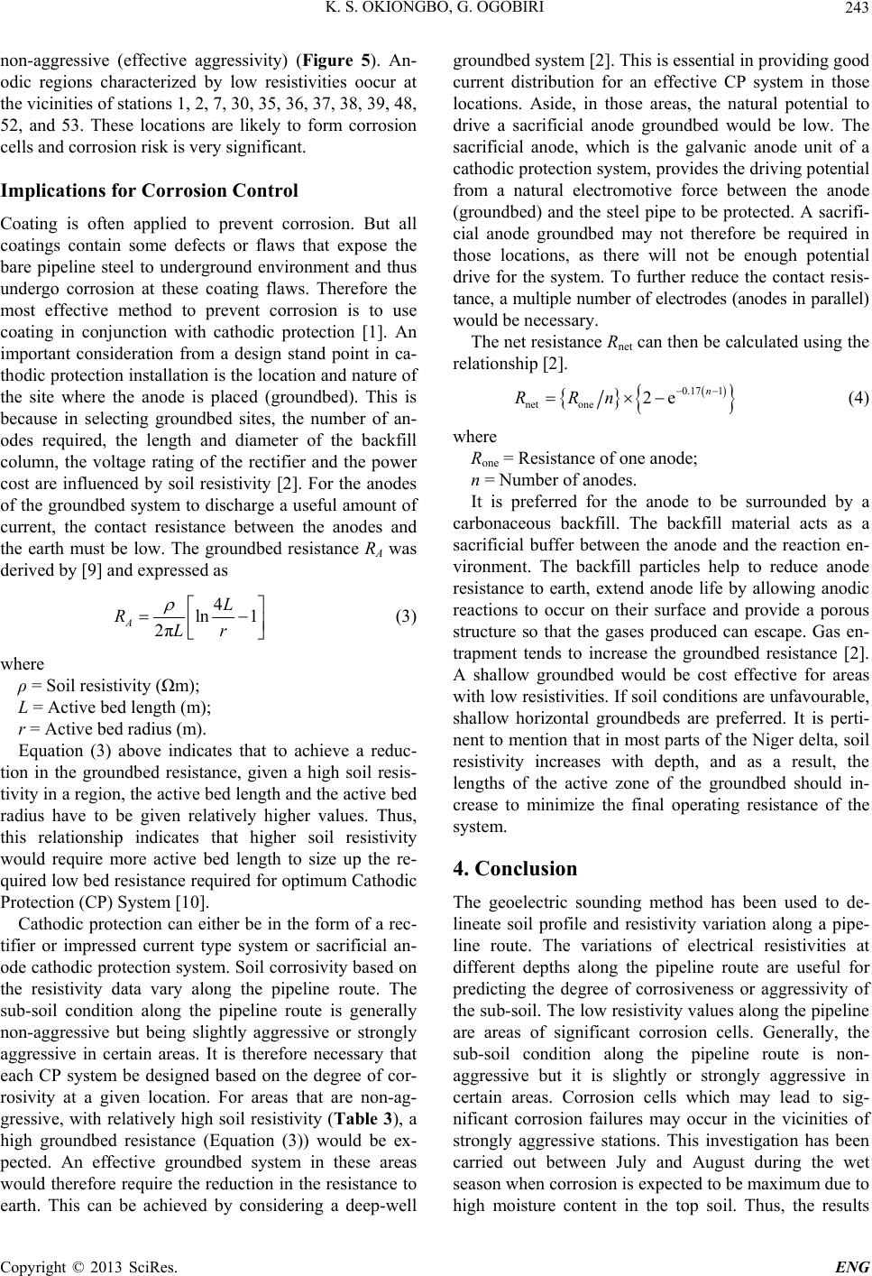

K. S. OKIONGBO, G. OGOBIRI 243

non-aggressive (effective aggressivity) (Figure 5). An-

odic regions characterized by low resistivities oocur at

the vicinities of stations 1, 2, 7, 30, 35, 36, 37, 38, 39, 48,

52, and 53. These locations are likely to form corrosion

cells and corrosion risk is very significant.

Implications for Corrosion Control

Coating is often applied to prevent corrosion. But all

coatings contain some defects or flaws that expose the

bare pipeline steel to underground environment and thus

undergo corrosion at these coating flaws. Therefore the

most effective method to prevent corrosion is to use

coating in conjunction with cathodic protection [1]. An

important consideration from a design stand point in ca-

thodic protection installation is the location and nature of

the site where the anode is placed (groundbed). This is

because in selecting groundbed sites, the number of an-

odes required, the length and diameter of the backfill

column, the voltage rating of the rectifier and the power

cost are influenced by soil resistivity [2]. For the anodes

of the groundbed system to discharge a useful amount of

current, the contact resistance between the anodes and

the earth must be low. The groundbed resistance RA was

derived by [9] and expressed as

ln 1

2

RLr

















(3)

where

ρ = Soil resistivity (m);

L = Active bed length (m);

r = Active bed radius (m).

Equation (3) above indicates that to achieve a reduc-

tion in the groundbed resistance, given a high soil resis-

tivity in a region, the active bed length and the active bed

radius have to be given relatively higher values. Thus,

this relationship indicates that higher soil resistivity

would require more active bed length to size up the re-

quired low bed resistance required for optimum Cathodic

Protection (CP) System [10].

Cathodic protection can either be in the form of a rec-

tifier or impressed current type system or sacrificial an-

ode cathodic protection system. Soil corrosivity based on

the resistivity data vary along the pipeline route. The

sub-soil condition along the pipeline route is generally

non-aggressive but being slightly aggressive or strongly

aggressive in certain areas. It is therefore necessary that

each CP system be designed based on the degree of cor-

rosivity at a given location. For areas that are non-ag-

gressive, with relatively high soil resistivity (Table 3), a

high groundbed resistance (Equation (3)) would be ex-

pected. An effective groundbed system in these areas

would therefore require the reduction in the resistance to

earth. This can be achieved by considering a deep-well

groundbed system [2]. This is essential in providing good

current distribution for an effective CP system in those

locations. Aside, in those areas, the natural potential to

drive a sacrificial anode groundbed would be low. The

sacrificial anode, which is the galvanic anode unit of a

cathodic protection system, provides the driving potential

from a natural electromotive force between the anode

(groundbed) and the steel pipe to be protected. A sacrifi-

cial anode groundbed may not therefore be required in

those locations, as there will not be enough potential

drive for the system. To further reduce the contact resis-

tance, a multiple number of electrodes (anodes in parallel)

would be necessary.

The net resistance Rnet can then be calculated using the

relationship [2].









0.17 1

net one2e n

RRn 

 (4)

where

Rone = Resistance of one anode;

n = Number of anodes.

It is preferred for the anode to be surrounded by a

carbonaceous backfill. The backfill material acts as a

sacrificial buffer between the anode and the reaction en-

vironment. The backfill particles help to reduce anode

resistance to earth, extend anode life by allowing anodic

reactions to occur on their surface and provide a porous

structure so that the gases produced can escape. Gas en-

trapment tends to increase the groundbed resistance [2].

A shallow groundbed would be cost effective for areas

with low resistivities. If soil conditions are unfavourable,

shallow horizontal groundbeds are preferred. It is perti-

nent to mention that in most parts of the Niger delta, soil

resistivity increases with depth, and as a result, the

lengths of the active zone of the groundbed should in-

crease to minimize the final operating resistance of the

system.

4. Conclusion

The geoelectric sounding method has been used to de-

lineate soil profile and resistivity variation along a pipe-

line route. The variations of electrical resistivities at

different depths along the pipeline route are useful for

predicting the degree of corrosiveness or aggressivity of

the sub-soil. The low resistivity values along the pipeline

are areas of significant corrosion cells. Generally, the

sub-soil condition along the pipeline route is non-

aggressive but it is slightly or strongly aggressive in

certain areas. Corrosion cells which may lead to sig-

nificant corrosion failures may occur in the vicinities of

strongly aggressive stations. This investigation has been

carried out between July and August during the wet

season when corrosion is expected to be maximum due to

high moisture content in the top soil. Thus, the results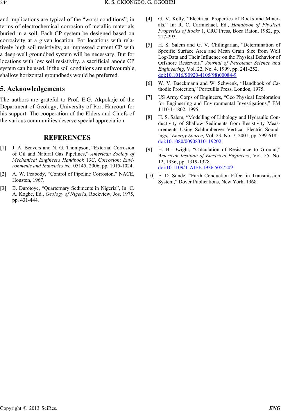

K. S. OKIONGBO, G. OGOBIRI

244

and implications are typical of the “worst conditions”, in

terms of electrochemical corrosion of metallic materials

buried in a soil. Each CP system be designed based on

corrosivity at a given location. For locations with rela-

tively high soil resistivity, an impressed current CP with

a deep-well groundbed system will be necessary. But for

locations with low soil resistivity, a sacrificial anode CP

system can be used. If the soil conditions are unfavourable,

shallow horizontal groundbeds would be preferred.

5. Acknowledgements

The authors are grateful to Prof. E.G. Akpokoje of the

Department of Geology, University of Port Harcourt for

his support. The cooperation of the Elders and Chiefs of

the various communities deserve special appreciation.

REFERENCES

[1] J. A. Beavers and N. G. Thompson, “External Corrosion

of Oil and Natural Gas Pipelines,” American Society of

Mechanical Engineers Handbook 13C, Corrosion: Envi-

ronments and Industries No. 05145, 2006, pp. 1015-1024.

[2] A. W. Peabody, “Control of Pipeline Corrosion,” NACE,

Houston, 1967.

[3] B. Durotoye, “Quarternary Sediments in Nigeria”, In: C.

A. Kogbe, Ed., Geology of Nigeria, Rockview, Jos, 1975,

pp. 431-444.

[4] G. V. Kelly, “Electrical Properties of Rocks and Miner-

als,” In: R. C. Carmichael, Ed., Handbook of Physical

Properties of Rocks 1, CRC Press, Boca Raton, 1982, pp.

217-293.

[5] H. S. Salem and G. V. Chilingarian, “Determination of

Specific Surface Area and Mean Grain Size from Well

Log-Data and Their Influence on the Physical Behavior of

Offshore Reservoir,” Journal of Petroleum Science and

Engineering, Vol. 22, No. 4, 1999, pp. 241-252.

doi:10.1016/S0920-4105(98)00084-9

[6] W. V. Baeckmann and W. Schwenk, “Handbook of Ca-

thodic Protection,” Portcullis Press, London, 1975.

[7] US Army Corps of Engineers, “Geo Physical Exploration

for Engineering and Environmental Investigations,” EM

1110-1-1802, 1995.

[8] H. S. Salem, “Modelling of Lithology and Hydraulic Con-

ductivity of Shallow Sediments from Resistivity Meas-

urements Using Schlumberger Vertical Electric Sound-

ings,” Energy Source, Vol. 23, No. 7, 2001, pp. 599-618.

doi:10.1080/00908310119202

[9] H. B. Dwight, “Calculation of Resistance to Ground,”

American Institute of Electrical Engineers, Vol. 55, No.

12, 1936, pp. 1319-1328.

doi:10.1109/T-AIEE.1936.5057209

[10] E. D. Sunde, “Earth Conduction Effect in Transmission

System,” Dover Publications, New York, 1968.