Cyclic Operator Decomposition for Solving the Differential Equations

doi:10.4236/apm.2013.31A025

Paper Menu >>

Journal Menu >>

Advances in Pure Mathematics, 2013, 3, 178-182

http://dx.doi.org/10.4236/apm.2013.31A025 Published Online January 2013 (http://www.scirp.org/journal/apm)

Cyclic Operator Decomposition for Solving the

Differential Equations

Ivan Gonoskov

Institute of Applied Physics of the Russian Academy of Sciences, Nizhny Novgorod, Russia

Email: [email protected]

Received October 19, 2012; revised November 23, 2012; accepted December 6, 2012

ABSTRACT

We present an approach how to obtain solutions of arbitrary linear operator equation for unknown functions. The par-

ticular solution can be represented by the infinite operator series (Cyclic Operator Decomposition), which acts the gen-

erating function. The method allows us to choose the cyclic operators and corresponding generating function selectively,

depending on initial problem for analytical or numerical study. Our approach includes, as a particular case, the pertur-

bation theory, but generally does not require inside any small parameters and unperturbed solutions. We demonstrate

the applicability of the method to the analysis of several differential equations in mathematical physics, namely, classi-

cal oscillator, Schrödinger equation, and wave equation in dispersive medium.

Keywords: Operator Decomposition; Spectral Theory; Propagator

1. Introduction

Various classical and quantum-mechanical problems in

theoretical physics lead to the necessity of solving the

linear operator equations for unknown functions and, in

particular, the differential equations. Exact non-trivial

analytical solutions of these equations, which include

finite combinations of elementary operations and special

functions, are known only for a number of specific cases.

However, there are many actual and important cases for

which such exact solutions were not still obtained even

by using severe approximations for the corresponding

interaction operators. For the cases when exact solutions

are unknown, some approximate methods are usually

used. They can be conventionally divided into two types:

1) varieties of perturbation theory and 2) numerical cal-

culations (which generally are also based on perturbation

theory). In spite of significant usefulness and applicabil-

ity, these methods are not free from various limitations

and disadvantages. The perturbation theory approaches

may lead to divergent series, they need sometimes suit-

able unperturbed solutions, and, finally, they do not pro-

vide even estimations for precision in most cases (see

[1,2] and references therein). On the other hand, numeri-

cal schemes, which are from the very beginning ap-

proximate, usually also do not give reliable estimations

for the precision (some reasonings can be found in [3,4]).

Moreover, they can hardly give an asymptotic behavior

of the solutions at infinity. Thus, the development of the

general method which allows to overcome some of the

above-mentioned difficulties is the main object of our

study.

In this manuscript we develop an approach based on

the theory of Cyclic Operator Decomposition (COD),

which gives the opportunities to obtain solutions (exact

or approximate) of the differential equations with arbi-

trary operators. The particular solution can be repre-

sented by the infinite cyclic operators series, which acts

the previously determined generating function. The cy-

clic operators and the corresponding generating function

(COD components) can be specified through the given

operators in the differential equation. Under the conver-

gence requirement, these COD components can be cho-

sen in different ways depending on the certain problem

statement. The procedure differs from the using of Born

series (or corresponding Neumann series) in the pertur-

bation theory [5-8] and S-matrix theory of Heisenberg,

Feynmann and Dyson [9]. It can be understood easily by

studying, for example, the difference between the formal

definition of the generating function and Green’s func-

tion (the last one is derived in some cases by using the

operator resolvent formalism) [5,7,10-12]. Generally, the

proposed series does not require any small parameters or

unperturbed solutions for the convergence. But, as a

matter of fact, the procedure can be transformed, under

some certain choice of COD components, to the “stan-

dard” perturbation theory with small parameters. For the

potentials without strong singularities, with reasonable

I. GONOSKOV 179

choice of the cyclic operators and generating function,

the corresponding series usually has uniform conver-

gence. Some additional features and advantages of our

approach for analytical and numerical solving the differ-

ential equations are demonstrated in sections below.

2. Theory of Cyclic Operator Decomposition

Let us start from the general case of operator equation for

unknown function:

ˆ0.D





(1)

Here is an arbitrary given linear operator and



is an unknown function, which can be a vector or matrix

of arbitrary dimensionality. This equation can lead in

particular cases to arbitrary linear differential equations,

which are considered in examples below.

Let us consider a pair of operators and V, which

are determined by the following condition:

Gˆ

ˆˆ

.DG

V

ˆˆ

at: ;GGGI





hat: 0,



 

(2)

Since the choice of this pair is partly optional, we

impose additional conditions on the operator :

h (3)

0, t





 (4)

where

is the identity operator. Any function



which satisfies Equation (4), will be called generating

function. Now we can write the following equation:





ˆˆ.

IGV







(5)

As we can check, under the above-mentioned condi-

tions for and



, any solution of Equation (5) ful-

fills Equation (1). Equation (5) can be solved in terms of

the following Cyclic Operator Decomposition:



ˆˆˆ

ˆˆ

IGVGV

IGV















ˆˆ











 











 (6)

This is the exact particular solution of Equation (1)

with corresponding particular COD components deter-

mined by Equations (2) and (3). The solution makes

sense only if the obtained series is convergent. This can

be achieved in different cases depending on and



, for example, if we work in Banach space and corre-

sponding operator norm is 1

ˆˆ1GV



ˆ,D

. The convergence

of some similar operator series was considered also in

[5,13].

The theory can be easily generalized also to the case of

the equations with given sources:







(7)

where an arbitrary given function



describes the arbi-

trary sources. The unknown function



could be found

naturally if the inverse operator is known: 1









D

 

ˆˆ

ˆˆn

IGV G

However, the inverse operator can not be easily

found for a number of problems. Then, we can write a

solution of this equation analogously by using COD:









 







(8)

In contrast to the case of Equation (1), now we can

choose



for some non-trivial particular solutions.



Then we can obtain the particular solution of Equation

(7), which corresponds to the following particular deter-

mination of the inverse operator in terms of COD:



111

ˆˆ

DI GVG

















(9)

Important feature of the proposed theory is that, while

the conditions Equations (3) and (4) should be fulfilled

and the convergence of the series is necessary, we still

have a great freedom of choosing and corresponding

. Generally, it gives us opportunities to obtain all the



possible solutions of Equation (1). Sometimes we can

naturally choose and



in accordance, for exam-

ple, with the corresponding initial conditions for Cauchy

problem or boundary conditions for boundary-value

problems.

In some cases, the exact solution Equation (6) can be

used naturally for obtaining the approximate solution

with finite number of terms. It can be done, for example,

when, starting from certain number n, the following con-





ˆˆ

GV GV









ditions are satisfied: .

These are the sufficient conditions enabling one to derive

the approximate solution with the prescribed accuracy.

Further, the proposed method provides another advantage

if one performs numerical calculations. According to the

exact solution Equation (6), we can use recurrent rela-

tions when calculating numerically the approximate solu-

tions. In this case, the calculation of any next term in the

corresponding series does not require more numerical

resources than the calculation of the previous one.

3. Examples

In this section we apply the proposed theory of Cyclic

Operator Decomposition for the various cases of differ-

ential equations. Let us first consider the Cauchy prob-

lem for the equation of classical oscillator. Note that this

equation, if written in other variables, is the stationary

one-dimensional Schrödinger equation with given energy,

and it can be transformed also to the Riccati equation by

using logarithmic substitution.

I. GONOSKOV

180



20,

ftf













(10)

where





is an unknown function, is an ar-

bitrary time-dependent frequency and a, b are arbitrary

constants. Here, it is natural to choose the components

for COD as follows:



, .

btt

GVt









ˆdd















(11)

If we fix (by our local convention, which we will use

below) that we write for brevity the same variable upper

limit of integration as the integration variable and deter-

mine the successive integration (step by step from right

to left), we can write a simple expression for the solution:



 

ab ab

tt tt

tabttt ta

ttttta





 

 

 





 

bttt



















(12)

It is important to note now, that the presented series

(Equation (12)) has rapid uniform convergence at least in

any interval, where is bounded. For example, in

the limited interval



0,t



the rate of convergence for

can be estimated in the following way (we assume

here for simplicity, that ab



0b, , and the

maximum of





in the corresponding interval is

max



max

-thtermofseries. (13)

In the same way, the convergence can be demonstrated

for other different COD’s, when the cyclic operators are

bounded for the given generating functions in the given

relevant interval. Moreover, if additionally







 



0t

is a

real function, and , we have a

decreasing alternating series for the above example, and

we can estimate the precision of partial sum of the series

by the value of the last term.



t00

Now we focus on some particular cases of







. To

demonstrate that it is possible to obtain a solution with

any prescribed precision, we consider a case when





1sin 0



 





1a0b



and , , . Calculation of the first

two terms in Equation (12) gives

tt



1sin

ftt tt.







 





0.0273

(14)

By calculating the third term in Equation (12), we

obtain



if we consider t in the interval [0,1].



Sometimes we can find also the asymptotic behavior

of the solution. As an example, we consider the case





2tt



0 and ab

tt1a0b, , , where







an arbitrary constant, 1





  

. Using again Equation (12)

we obtain exact solution in the following form:

 

112

122324





 



  (15)



 





0t

  

By analyzing the corresponding series we can obtain a

simple upper estimate for the solution :

1exp,

12 2



 







 

 





:t



(16)

which gives us the following asymptotic behavior at

exp .

















(17)

In this case, the same asymptotic can be found also

from WKB theory (see, for example, quasiclassical ap-

proximation in [14,15]).

Let us now demonstrate the selective choice of cyclic

operators. For that we consider stationary one-dimen-

sional Schrödinger equation (we use below the units

where



1





2e0,

EA x









 





(18)





where



2Em1

is an unknown function, which describes

quantum state with energy E in the continuum; A, β are

arbitrary real constants. Without loss of generality (one

can use scale transformations of Equation (18)) we can

assume ,





. To find the solution of this

equation, we can choose the components for COD in

different ways. For example, if one interests in the be-

havior of







0x near



and in small values of E,

he can choose



G

and use nearly the same tech-

nique as in Equations (11) and (12). However, this choice

can be inconvenient for the analysis of the long-range

behavior. Another variant of choosing the components

for COD is the following (we use also Equation (9) for

the particular determination of ):

I. GONOSKOV 181



000

ˆ,e

ˆˆˆˆ

ˆdd,

Gmx C

GGV

GxxV











 

 

















ˆˆ

, e,

imx imx

mVA









eimx









(19)

where C1 and C2 are arbitrary constants. To obtain the

general solution, we consider the particular case of gen-

erating function and corresponding par-

ticular solution



. Then we derive by using a rule

of infinite geometric series:



im x

kimx



















ˆˆ

im x

GV xGV





























 













(20)

From here we obtain



2ki









2pp

e1 e

imxn nx









 





 (21)

and the general solution in the following form:

 



 Cx





 (22)

The corresponding series converges at any A and real

In a similar way we can obtain solutions for multi-

dimensional equations. Let us consider the stationary

Schrödinger equation with potential surface





Ur, m-

dimensional Laplace operator ∆, and energy E:

ulti



20.











 

 (23)

Then we can choose







EUr

ˆˆ

GV , and



is any solution of 0



. From corresponding

COD we can obtain a solution:



1VV







 



r10.





 





1 2

(24)

The inverse Laplace operator can be written, for ex-

ample, as 1



ˆ

, where

is the Fourier

transform operator and k is an absolute value of the wave

vector in this transform.

Another choice of COD components can be better for

the finding of the bound states with . We can

0E



2Ur

choose: ,

GEˆ

2,V



is any solution of







 0, and write the inverse operator 1



for

COD as follows:

ˆˆˆ

GE FF





 (25)

In this way, we can calculate in some cases the terms

in the corresponding COD by evaluating the poles at

imaginary values 2

kiE .

Now we consider time-dependent three-dimensional

Schrödinger equation to demonstrate other applications

of the proposed method. Let us consider propagation of

charged particle with arbitrary electromagnetic interactions

(below





r1qc

is the vector potential, and ):







1,,,0.

ii tUtt









 







Arr r (26)

Here, we can choose the components for COD in a

variety of ways depending on peculiar properties of the

interactions. One special choice is the following:



ˆ,(,) ,

ˆd,

ˆ,,,

Gi t

Git

Vi tUt

 





 





 



Ar r

 

000

ˆˆˆ

,1 ddd.

ttt

titVitVtV













rr

(27)

where corresponds to the time-dependent Hamilto-

nian. It gives the following solution:

(28)

This solution can be useful for the numerical calcula-

tions, namely, for the finding the propagator , which

gives:











ttP tOt



 rr



ˆ,tr



, see also [4] and

references therein. If we use additionally internal time-

ordering, we can transform this expression to Dyson se-

ries (see [9,16]).

Finally, we consider the wave equation for electro-

magnetic waves in dispersive medium. We assume that

an arbitrarily given operator  which describes

electric dispersion does not depend nonlinearly on the

field, i.e. we still have linear problem. In this case the

equation for unknown vector potential

r is the

following (see for example [17]):

 

ˆ,,0,

 



 











rAr



(29)

with the initial conditions

















SrRr (30)

We can choose the following components for COD: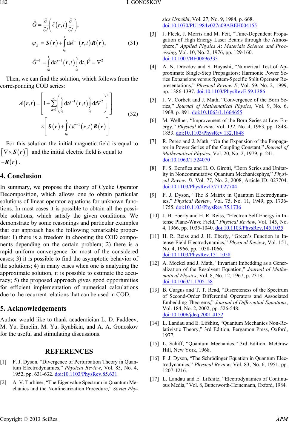

I. GONOSKOV

182



ˆˆ





















d, ,

ttV











rRr





d, .



























r Rr









(31)

Then, we can find the solution, which follows from the

corresponding COD series:



,1 d













 

















(32)

For this solution the initial magnetic field is equal to



Rr

and the initial electric field is equal to

4. Conclusion

In summary, we propose the theory of Cyclic Operator

Decomposition, which allows one to obtain particular

solutions of linear operator equations for unknown func-

tions. In most cases it is possible to obtain all the possi-

ble solutions, which satisfy the given conditions. We

demonstrate by some reasonings and particular examples

that our approach has the following remarkable proper-

ties: 1) there is a freedom in choosing the COD compo-

nents depending on the certain problem; 2) there is a

rapid uniform convergence for most of the considered

cases; 3) it is possible to find the asymptotic behavior of

the solutions; 4) in many cases when one is analyzing the

approximate solution, it is possible to estimate the accu-

racy; 5) the proposed approach gives good opportunities

for efficient implementation of numerical calculations

due to the recurrent relations that can be used in COD.

5. Acknowledgements

Author would like to thank academician L. D. Faddeev,

M. Yu. Emelin, M. Yu. Ryabikin, and A. A. Gonoskov

for the useful and stimulating discussions.

REFERENCES

[1] F. J. Dyson, “Divergence of Perturbation Theory in Quan-

tum Electrodynamics,” Physical Review, Vol. 85, No. 4,

1952, pp. 631-632. doi:10.1103/PhysRev.85.631

[2] A. V. Turbiner, “The Eigenvalue Spectrum in Quantum Me-

chanics and the Nonlinearization Procedure,” Soviet Phy-

sics Uspekhi, Vol. 27, No. 9, 1984, p. 668.

doi:10.1070/PU1984v027n09ABEH004155

[3] J. Fleck, J. Morris and M. Feit, “Time-Dependent Propa-

gation of High Energy Laser Beams through the Atmos-

phere,” Applied Physics A: Materials Science and Proc-

essing, Vol. 10, No. 2, 1976, pp. 129-160.

doi:10.1007/BF00896333

[4] A. N. Drozdov and S. Hayashi, “Numerical Test of Ap-

proximate Single-Step Propagators: Harmonic Power Se-

ries Expansions versus System-Specific Split Operator Re-

presentations,” Physical Review E, Vol. 59, No. 2, 1999,

pp. 1386-1397. doi:10.1103/PhysRevE.59.1386

[5] J. V. Corbett and J. Math, “Convergence of the Born Se-

ries,” Journal of Mathematical Physics, Vol. 9, No. 6,

1968, p. 891. doi:10.1063/1.1664655

[6] M. Wellner, “Improvement of the Born Series at Low En-

ergy,” Physical Review, Vol. 132, No. 4, 1963, pp. 1848-

1853. doi:10.1103/PhysRev.132.1848

[7] R. Perez and J. Math, “On the Expansion of the Propaga-

tor in Power Series of the Coupling Constant,” Journal of

Mathematical Physics, Vol. 20, No. 2, 1979, p. 241.

doi:10.1063/1.524070

[8] F. S. Bemfica and H. O. Girotti, “Born Series and Unitar-

ity in Noncommutative Quantum Mechanicsphys,” Physi-

cal Review D, Vol. 77, No. 2, 2008, Article ID: 027704.

doi:10.1103/PhysRevD.77.027704

[9] F. J. Dyson, “The S Matrix in Quantum Electrodynam-

ics,” Physical Review, Vol. 75, No. 11, 1949, pp. 1736-

1755. doi:10.1103/PhysRev.75.1736

[10] J. H. Eberly and H. R. Reiss, “Electron Self-Energy in In-

tense Plane-Wave Field,” Physical Review, Vol. 145, No.

4, 1966, pp. 1035-1040. doi:10.1103/PhysRev.145.1035

[11] H. R. Reiss and J. H. Eberly, “Green’s Function in In-

tense-Field Electrodynamics,” Physical Review, Vol. 151,

No. 4, 1966, pp. 1058-1066.

doi:10.1103/PhysRev.151.1058

[12] A. Mockel and J. Math, “Invariant Imbedding as a Gener-

alization of the Resolvent Equation,” Journal of Mathe-

matical Physics, Vol. 8, No. 12, 1967, p. 2318.

doi:10.1063/1.1705158

[13] B. Ćurgus and T. T. Read, “Discreteness of the Spectrum

of Second-Order Differential Operators and Associated

Embedding Theorems,” Journal of Differential Equations,

Vol. 184, No. 2, 2002, pp. 526-548.

doi:10.1006/jdeq.2001.4152

[14] L. Landau and E. Lifshitz, “Quantum Mechanics Non-Re-

lativistic Theory,” 3rd Edition, Pergamon Press, Oxford,

1977.

[15] L. Schiff, “Quantum Mechanics,” 3rd Edition, McGraw

Hill, New York, 1968.

[16] F. J. Dyson, “The Schrödinger Equation in Quantum Elec-

trodynamics,” Physical Review, Vol. 83, No. 6, 1951, pp.

1207-1216.

[17] L. Landau and E. Lifshitz, “Electrodynamics of Continu-

ous Media,” Vol. 8, Butterworth-Heinemann, Oxford, 1984.