Orthogonal optimization of horizontal well fracturing method

doi:10.4236/ns.2010.29126

Paper Menu >>

Journal Menu >>

Vol.2, No.9, 1030-1034 (2010) Natural Science

http://dx.doi.org/10.4236/ns.2010.29126

Orthogonal optimization of horizontal well fracturing

method

Chi Dong*, Kao-Ping Song, Xiao-Qi Chen

Key Laboratory of Ministry of China on Enhanced Oil and Gas Recovery, Da Qing, China;

*Corresponding Author: [email protected]

Received 18 May 2010; revised 29 June 2010; accepted 5 July 2010.

ABSTRACT

In many applications, streamline simulation sh-

ows particular advantages over finite-difference

simulation. By the advantages of streamline

simulation such as its ability to display paths of

fluid flow and acceleration factor in simulation,

the description of flooding process gets more

visual effect. The communication between wells

and flooding area has been represented appro-

priately. In low permeability reservoirs horizon-

tal wells have been applied to stimulate. And

some horizontal wells have been fractured. But

different fracturing methods are followed by

different effects. Through streamline simulation

this paper presents that the fractures improve

both the productivity of horizontal well and the

efficiency of the flooding unit. And the syntag-

matic relation of distance between artificial frac-

tures, fracture length and fracture conductivity

has been given by orthogonal experiment. This

method has been applied to the D160 reservoir

in Daqing Oilfield. The production history of this

reservoir is about 2 years. The reservoir is main-

tained above bubble point so the simulation

meets the slight compressibility assumption.

New horizontal wells are fractured followed from

this rule.

Keywords: Streamline Simulation; Horizontal Well;

Optimization

1. INTRODUCTION

Using horizontal wells to stimulate and enhance oil re-

covery, has been applied widely all over the world. It is

necessary to use horizontal wells to develop low perme-

ability reservoirs. In the long process of practice, it was

discovered that the advantages of horizontal well would

not be made full use of when only the horizontal well

drilling techniques not the combination with the actual

development conditions has be paid attention to. In low

permeability reservoirs the horizontal wells need to be

fractured to stimulate. As the increase of the length of

horizontal section, the number of artificial fractures

should be increased too. And the syntagmatic relation of

distance between fractures, fracture length and fracture

conductivity is necessary to be optimized.

As the application of high-resolution geologic models

in simulations, more attention had been paid to the use

of simulation in oil field development. Finite difference

method which applied widely cannot meet the needs

such as high computational efficiency and being visually

appealing. So the 3D streamline simulation approach has

been applied to simulation as complementary to finite

difference simulation techniques [1-4].

Streamline simulation is in the advanced and matured

stage in slightly compressible system. It calculates the

saturation via 1D streamline instead of saturation field

[5]. Both computational efficiency and matching high

resolution geologic models becomes possible. Not like

the unity of the saturation in finite difference grid cell,

streamline simulation provides several values of the

saturation in one grid cell, then the fineness of the solu-

tion gets elevated.

Taking advantage of streamline simulation’s particular

capability, the syntagmatic relation of distance between

artificial fractures, fracture length and fracture conduc-

tivity has been optimized by orthogonal experiment

method.

2. STREAMLINE SIMULATION THEORY

2.1. Velocity Field Solution and Streamline

Tracing

The streamline model is a model with the assumptions as

follows: 1) Considering the effects of gravity and capil-

lary; 2) There are oil phase and water phase in the res-

ervoir; 3) The fluid flow in the reservoir is incompressi-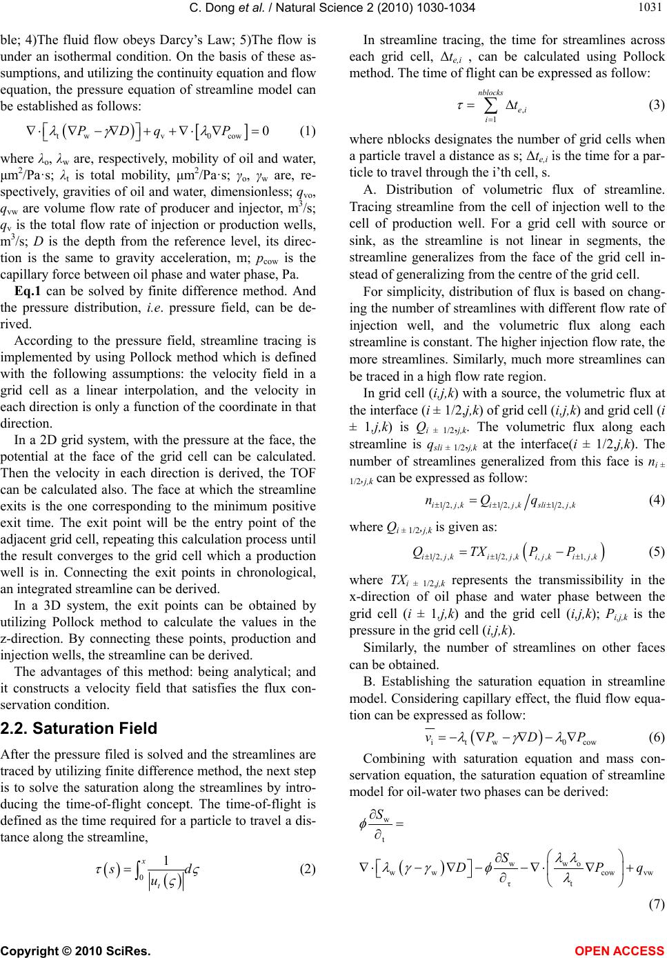

C. Dong et al. / Natural Science 2 (2010) 1030-1034

103

1031

ble; 4)The fluid flow obeys Darcy’s Law; 5)The flow is

under an isothermal condition. On the basis of these as-

sumptions, and utilizing the continuity equation and flow

equation, the pressure equation of streamline model can

be established as follows:







twv 0cow

0PDqP

 



 

 (1)

where λo, λw are, respectively, mobility of oil and water,

μm2/Pa·s; λt is total mobility, μm2/Pa·s; γo, γw are, re-

spectively, gravities of oil and water, dimensionless; qvo,

qvw are volume flow rate of producer and injector, m3/s;

qv is the total flow rate of injection or production wells,

m3/s; D is the depth from the reference level, its direc-

tion is the same to gravity acceleration, m; pcow is the

capillary force between oil phase and water phase, Pa.

Eq.1 can be solved by finite difference method. And

the pressure distribution, i.e. pressure field, can be de-

rived.

According to the pressure field, streamline tracing is

implemented by using Pollock method which is defined

with the following assumptions: the velocity field in a

grid cell as a linear interpolation, and the velocity in

each direction is only a function of the coordinate in that

direction.

In a 2D grid system, with the pressure at the face, the

potential at the face of the grid cell can be calculated.

Then the velocity in each direction is derived, the TOF

can be calculated also. The face at which the streamline

exits is the one corresponding to the minimum positive

exit time. The exit point will be the entry point of the

adjacent grid cell, repeating this calculation process until

the result converges to the grid cell which a production

well is in. Connecting the exit points in chronological,

an integrated streamline can be derived.

In a 3D system, the exit points can be obtained by

utilizing Pollock method to calculate the values in the

z-direction. By connecting these points, production and

injection wells, the streamline can be derived.

The advantages of this method: being analytical; and

it constructs a velocity field that satisfies the flux con-

servation condition.

2.2. Saturation Field

After the pressure filed is solved and the streamlines are

traced by utilizing finite difference method, the next step

is to solve the saturation along the streamlines by intro-

ducing the time-of-flight concept. The time-of-flight is

defined as the time required for a particle to travel a dis-

tance along the streamline,

 





 (2)

In streamline tracing, the time for streamlines across

each grid cell, Δte,i , can be calculated using Pollock

method. The time of flight can be expressed as follow:

nblocks







 (3)

where nblocks designates the number of grid cells when

a particle travel a distance as s; Δte,i is the time for a par-

ticle to travel through the i’th cell, s.

A. Distribution of volumetric flux of streamline.

Tracing streamline from the cell of injection well to the

cell of production well. For a grid cell with source or

sink, as the streamline is not linear in segments, the

streamline generalizes from the face of the grid cell in-

stead of generalizing from the centre of the grid cell.

For simplicity, distribution of flux is based on chang-

ing the number of streamlines with different flow rate of

injection well, and the volumetric flux along each

streamline is constant. The higher injection flow rate, the

more streamlines. Similarly, much more streamlines can

be traced in a high flow rate region.

In grid cell (i,j,k) with a source, the volumetric flux at

the interface (i ± 1/2,j,k) of grid cell (i,j,k) and grid cell (i

± 1,j,k) is Qi ± 1/2,j,k. The volumetric flux along each

streamline is qsli ± 1/2,j,k at the interface(i ± 1/2,j,k). The

number of streamlines generalized from this face is ni ±

1/2,j,k can be expressed as follow:

12, ,12, ,12, ,ijk ijkslijk

nQq





(4)

where Qi ± 1/2,j,k is given as:



12, ,12, ,, ,1, ,i jkijkijkijk

QTXPP

 

 (5)

where TXi ± 1/2,j,k represents the transmissibility in the

x-direction of oil phase and water phase between the

grid cell (i ± 1,j,k) and the grid cell (i,j,k); Pi,j,k is the

pressure in the grid cell (i,j,k).

Similarly, the number of streamlines on other faces

can be obtained.

B. Establishing the saturation equation in streamline

model. Considering capillary effect, the fluid flow equa-

tion can be expressed as follow:





itw 0cow

vPDP



  (6)

Combining with saturation equation and mass con-

servation equation, the saturation equation of streamline

model for oil-water two phases can be derived:



wwo

ww cowvw

τt

DPq





 











 







(7)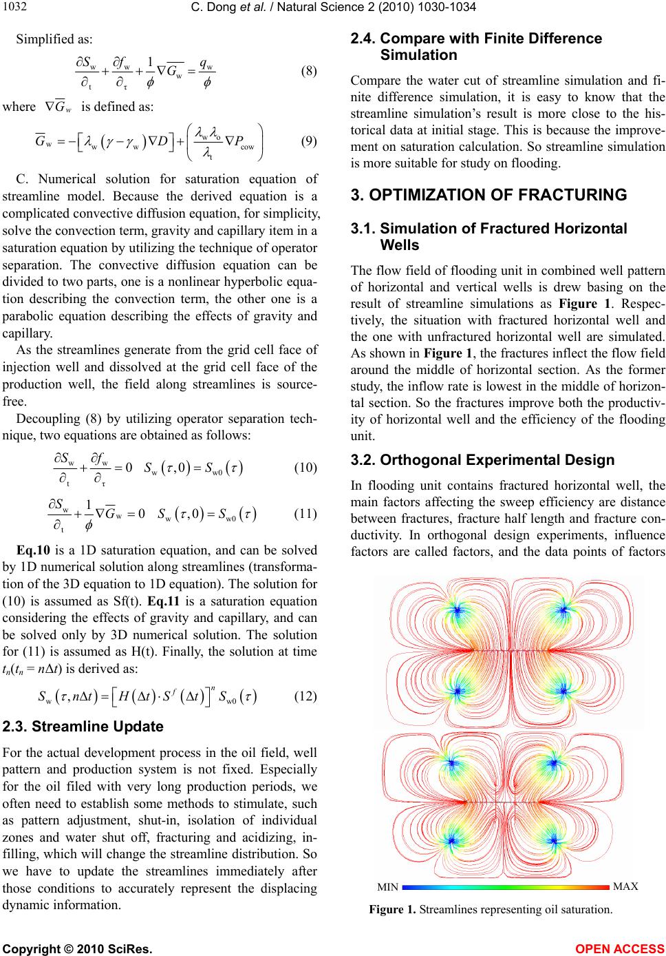

C. Dong et al. / Natural Science 2 (2010) 1030-1034

1032

Simplified as:

ww w

tτ

Sf q







 (8)

where w

G is defined as:



www cow

GDP



 





 







(9)

C. Numerical solution for saturation equation of

streamline model. Because the derived equation is a

complicated convective diffusion equation, for simplicity,

solve the convection term, gravity and capillary item in a

saturation equation by utilizing the technique of operator

separation. The convective diffusion equation can be

divided to two parts, one is a nonlinear hyperbolic equa-

tion describing the convection term, the other one is a

parabolic equation describing the effects of gravity and

capillary.

As the streamlines generate from the grid cell face of

injection well and dissolved at the grid cell face of the

production well, the field along streamlines is source-

free.

Decoupling (8) by utilizing operator separation tech-

nique, two equations are obtained as follows:

tτ

Sf





 

ww0

,0SS



 (10)



 







ww0

,0SS



 (11)

Eq.10 is a 1D saturation equation, and can be solved

by 1D numerical solution along streamlines (transforma-

tion of the 3D equation to 1D equation). The solution for

(10) is assumed as Sf(t). Eq.11 is a saturation equation

considering the effects of gravity and capillary, and can

be solved only by 3D numerical solution. The solution

for (11) is assumed as H(t). Finally, the solution at time

tn(tn = nΔt) is derived as:

 

ww0

SntHtStS





 



(12)

2.3. Streamline Update

For the actual development process in the oil field, well

pattern and production system is not fixed. Especially

for the oil filed with very long production periods, we

often need to establish some methods to stimulate, such

as pattern adjustment, shut-in, isolation of individual

zones and water shut off, fracturing and acidizing, in-

filling, which will change the streamline distribution. So

we have to update the streamlines immediately after

those conditions to accurately represent the displacing

dynamic information.

2.4. Compare with Finite Difference

Simulation

Compare the water cut of streamline simulation and fi-

nite difference simulation, it is easy to know that the

streamline simulation’s result is more close to the his-

torical data at initial stage. This is because the improve-

ment on saturation calculation. So streamline simulation

is more suitable for study on flooding.

3. OPTIMIZATION OF FRACTURING

3.1. Simulation of Fractured Horizontal

Wells

The flow field of flooding unit in combined well pattern

of horizontal and vertical wells is drew basing on the

result of streamline simulations as Figure 1. Respec-

tively, the situation with fractured horizontal well and

the one with unfractured horizontal well are simulated.

As shown in Figure 1, the fractures inflect the flow field

around the middle of horizontal section. As the former

study, the inflow rate is lowest in the middle of horizon-

tal section. So the fractures improve both the productiv-

ity of horizontal well and the efficiency of the flooding

unit.

3.2. Orthogonal Experimental Design

In flooding unit contains fractured horizontal well, the

main factors affecting the sweep efficiency are distance

between fractures, fracture half length and fracture con-

ductivity. In orthogonal design experiments, influence

factors are called factors, and the data points of factors

MIN MAX

Figure 1. Streamlines representing oil saturation.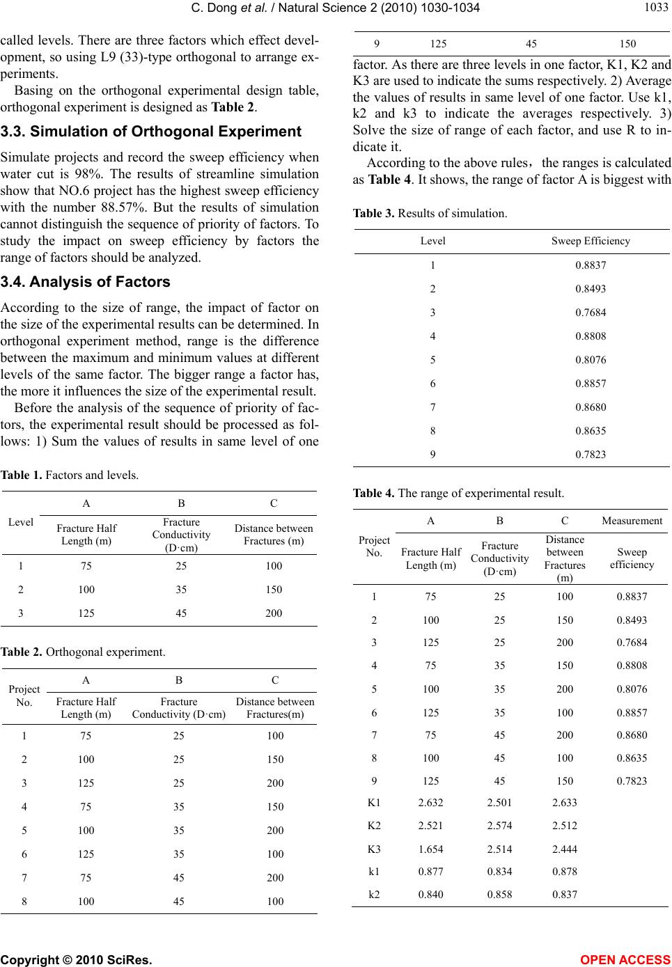

C. Dong et al. / Natural Science 2 (2010) 1030-1034

103

1033

called levels. There are three factors which effect devel-

opment, so using L9 (33)-type orthogonal to arrange ex-

periments.

Basing on the orthogonal experimental design table,

orthogonal experiment is designed as Table 2.

3.3. Simulation of Orthogonal Experiment

Simulate projects and record the sweep efficiency when

water cut is 98%. The results of streamline simulation

show that NO.6 project has the highest sweep efficiency

with the number 88.57%. But the results of simulation

cannot distinguish the sequence of priority of factors. To

study the impact on sweep efficiency by factors the

range of factors should be analyzed.

3.4. Analysis of Factors

According to the size of range, the impact of factor on

the size of the experimental results can be determined. In

orthogonal experiment method, range is the difference

between the maximum and minimum values at different

levels of the same factor. The bigger range a factor has,

the more it influences the size of the experimental result.

Before the analysis of the sequence of priority of fac-

tors, the experimental result should be processed as fol-

lows: 1) Sum the values of results in same level of one

Table 1. Factors and levels.

A B C

Level Fracture Half

Length (m)

Fracture

Conductivity

(D·cm)

Distance between

Fractures (m)

1 75 25 100

2 100 35 150

3 125 45 200

Table 2. Orthogonal experiment.

A B C

Project

No. Fracture Half

Length (m)

Fracture

Conductivity (D·cm)

Distance between

Fractures(m)

1 75 25 100

2 100 25 150

3 125 25 200

4 75 35 150

5 100 35 200

6 125 35 100

7 75 45 200

8 100 45 100

9 125 45 150

factor. As there are three levels in one factor, K1, K2 and

K3 are used to indicate the sums respectively. 2) Average

the values of results in same level of one factor. Use k1,

k2 and k3 to indicate the averages respectively. 3)

Solve the size of range of each factor, and use R to in-

dicate it.

According to the above rules，the ranges is calculated

as Table 4. It shows, the range of factor A is biggest with

Table 3. Results of simulation.

Level Sweep Efficiency

1 0.8837

2 0.8493

3 0.7684

4 0.8808

5 0.8076

6 0.8857

7 0.8680

8 0.8635

9 0.7823

Table 4. The range of experimental result.

A B C Measurement

Project

No. Fracture Half

Length (m)

Fracture

Conductivity

(D·cm)

Distance

between

Fractures

(m)

Sweep

efficiency

1 75 25 100 0.8837

2 100 25 150 0.8493

3 125 25 200 0.7684

4 75 35 150 0.8808

5 100 35 200 0.8076

6 125 35 100 0.8857

7 75 45 200 0.8680

8 100 45 100 0.8635

9 125 45 150 0.7823

K1 2.632 2.501 2.633

K2 2.521 2.574 2.512

K3 1.654 2.514 2.444

k1 0.877 0.834 0.878

k2 0.840 0.858 0.837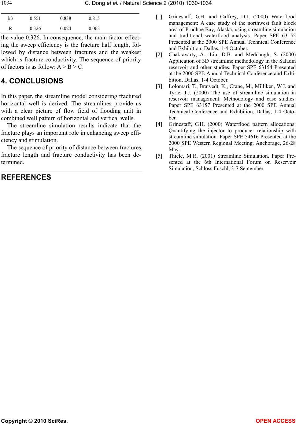

C. Dong et al. / Natural Science 2 (2010) 1030-1034

1034

k3 0.551 0.838 0.815

R 0.326 0.024 0.063

the value 0.326. In consequence, the main factor effect-

ing the sweep efficiency is the fracture half length, fol-

lowed by distance between fractures and the weakest

which is fracture conductivity. The sequence of priority

of factors is as follow: A > B > C.

4. CONCLUSIONS

In this paper, the streamline model considering fractured

horizontal well is derived. The streamlines provide us

with a clear picture of flow field of flooding unit in

combined well pattern of horizontal and vertical wells.

The streamline simulation results indicate that the

fracture plays an important role in enhancing sweep effi-

ciency and stimulation.

The sequence of priority of distance between fractures,

fracture length and fracture conductivity has been de-

termined.

REFERENCES

[1] Grinestaff, G.H. and Caffrey, D.J. (2000) Waterflood

management: A case study of the northwest fault block

area of Prudhoe Bay, Alaska, using streamline simulation

and traditional waterflood analysis. Paper SPE 63152

Presented at the 2000 SPE Annual Technical Conference

and Exhibition, Dallas, 1-4 October.

[2] Chakravarty, A., Liu, D.B. and Meddaugh, S. (2000)

Application of 3D streamline methodology in the Saladin

reservoir and other studies. Paper SPE 63154 Presented

at the 2000 SPE Annual Technical Conference and Exhi-

bition, Dallas, 1-4 October.

[3] Lolomari, T., Bratvedt, K., Crane, M., Milliken, W.J. and

Tyrie, J.J. (2000) The use of streamline simulation in

reservoir management: Methodology and case studies.

Paper SPE 63157 Presented at the 2000 SPE Annual

Technical Conference and Exhibition, Dallas, 1-4 Octo-

ber.

[4] Grinestaff, G.H. (2000) Waterflood pattern allocations:

Quantifying the injector to producer relationship with

streamline simulation. Paper SPE 54616 Presented at the

2000 SPE Western Regional Meeting, Anchorage, 26-28

May.

[5] Thiele, M.R. (2001) Streamline Simulation. Paper Pre-

sented at the 6th International Forum on Reservoir

Simulation, Schloss Fuschl, 3-7 September.